Image Classification using Swin Transformer

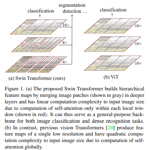
Swin Transformer by Microsoft researchers is a family of versatile transformer models adapted for vision tasks. They change the architectural approach compared to the original Vision Transformer model to get state-of-the-art results on various tasks. In this blog post, we will carry out image classification using Swin Transformer.

At the time of release, the authors published various results using the Swin Transformer model as the backbone. These include image classification, object detection, and image segmentation. However, in this blog post, we will only focus on fine-tuning the Swin Transformer model from Torchvision for image classification.

Our main objective is to train the model on a small dataset and get the best possible results.

What will we cover in this blog post?

• We will start with a discussion of the dataset. For fine-tuning the Swin Transformer model, we choose the food-101-tiny dataset.
• Then we will move to the coding part which consists of several sections:
  • First, we will cover the dataset preparation and writing the utility scripts.
  • Second, we will move on to the preparation of the Swin Transformer Tiny model.
  • Third, we will discuss the training script.
• After training the Swin Transformer model, we will use the trained model for inference on unseen data.

The Food-101 Tiny Dataset

We will use the Food-101-Tiny dataset from Kaggle for image classification using the Swin Transformer model in this blog post.

This is a much smaller version of the Food-101 dataset and contains only 10 classes instead of 101 classes. This serves two purposes:

• Our experimentation time with the model decreases substantially.
• And we get to know whether we can rely on Swin Transformer when we don’t have a huge dataset at hand.

The dataset contains a training and validation split and provides the following directory structure.

data/
└── food-101-tiny
    ├── train
    │   ├── apple_pie
    │   ├── bibimbap
    │   ├── cannoli
    │   ├── edamame
    │   ├── falafel
    │   ├── french_toast
    │   ├── ice_cream
    │   ├── ramen
    │   ├── sushi
    │   └── tiramisu
    └── valid
        ├── apple_pie
        ├── bibimbap
        ├── cannoli
        ├── edamame
        ├── falafel
        ├── french_toast
        ├── ice_cream
        ├── ramen
        ├── sushi
        └── tiramisu

It extracts into data/food-101-tiny folder which contains the splits and the respective class folder. There are 150 images for each class in the training set and 50 each in the validation set.

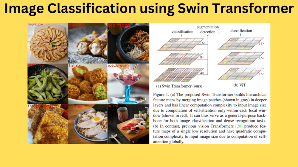
Here are some images from the dataset.

This should be a good starting point for using Swin Transformer for image classification.

Directory Structure

Before moving to the coding part, let’s take a look at the entire project’s directory structure.

├── input
│   ├── data
│   └── inference_data
├── outputs
│   ├── inference_results
│   ├── accuracy.png
│   ├── best_model.pth
│   ├── loss.png
│   └── model.pth
└── src
    ├── datasets.py
    ├── inference.py
    ├── model.py
    ├── train.py
    └── utils.py

• The input directory contains the data as we saw in the previous section. It also contains an inference_data directory with images for inference after training.
• The outputs directory contains all the results from training and inference including the trained weights.
• Finally, the src directory contains all the source code files.

Please make sure to download the dataset and arrange it according to the directory structure if you intend to run the training experiments.

All the inference data, source code files, and trained weights will be provided via the download section. You can directly run inference as well.

Image Classification using Swin Transformer

Let’s jump right into the coding part of the article.

All the Python source code files will remain inside the src directory.

Download Code

Helper Functions and Classes

We have a few helper functions and classes that will save the trained model and the loss & accuracy graphs for us. This code will go into the utils.py file.

import torch
import matplotlib
import matplotlib.pyplot as plt
import os

matplotlib.style.use('ggplot')

class SaveBestModel:
    """
    Class to save the best model while training. If the current epoch's 
    validation loss is less than the previous least less, then save the
    model state.
    """
    def __init__(
        self, best_valid_loss=float('inf')
    ):
        self.best_valid_loss = best_valid_loss
        
    def __call__(
        self, current_valid_loss, epoch, model, out_dir, name
    ):
        if current_valid_loss < self.best_valid_loss:
            self.best_valid_loss = current_valid_loss
            print(f"\nBest validation loss: {self.best_valid_loss}")
            print(f"\nSaving best model for epoch: {epoch+1}\n")
            torch.save({
                'epoch': epoch+1,
                'model_state_dict': model.state_dict(),
                }, os.path.join(out_dir, 'best_'+name+'.pth'))

def save_model(epochs, model, optimizer, criterion, out_dir, name):
    """
    Function to save the trained model to disk.
    """
    torch.save({
                'epoch': epochs,
                'model_state_dict': model.state_dict(),
                'optimizer_state_dict': optimizer.state_dict(),
                'loss': criterion,
                }, os.path.join(out_dir, name+'.pth'))

def save_plots(train_acc, valid_acc, train_loss, valid_loss, out_dir):
    """
    Function to save the loss and accuracy plots to disk.
    """
    # Accuracy plots.
    plt.figure(figsize=(10, 7))
    plt.plot(
        train_acc, color='tab:blue', linestyle='-', 
        label='train accuracy'
    )
    plt.plot(
        valid_acc, color='tab:red', linestyle='-', 
        label='validataion accuracy'
    )
    plt.xlabel('Epochs')
    plt.ylabel('Accuracy')
    plt.legend()
    plt.savefig(os.path.join(out_dir, 'accuracy.png'))
    
    # Loss plots.
    plt.figure(figsize=(10, 7))
    plt.plot(
        train_loss, color='tab:blue', linestyle='-', 
        label='train loss'
    )
    plt.plot(
        valid_loss, color='tab:red', linestyle='-', 
        label='validataion loss'
    )
    plt.xlabel('Epochs')
    plt.ylabel('Loss')
    plt.legend()
    plt.savefig(os.path.join(out_dir, 'loss.png'))

The SaveBestModel class saves the best model according to the lowest validation loss during training. It is invoked after each epoch. The save_model function saves the model after training. It also saves the optimizer state dictionary so that we can resume training if we wish to do so.

The save_plots function saves the accuracy and loss graphs to the disk which can be used for analysis.

Dataset Preparation

Next, we need scripts for preparing the PyTorch datasets and data loaders. The dataset already contains a training and a validation split. Furthermore, all the images are present inside their respective class folders. This makes our work a lot easier. The dataset preparation code will go into the datasets.py file.

import os

from torchvision import datasets, transforms
from torch.utils.data import DataLoader

# Required constants.
TRAIN_DIR = os.path.join('..', 'input', 'data', 'food-101-tiny', 'train')
VALID_DIR = os.path.join('..', 'input', 'data','food-101-tiny', 'valid')
IMAGE_SIZE = 224 # Image size of resize when applying transforms.
NUM_WORKERS = 4 # Number of parallel processes for data preparation.

# Training transforms
def get_train_transform(image_size):
    train_transform = transforms.Compose([
        transforms.Resize((image_size, image_size)),
        transforms.RandomHorizontalFlip(p=0.5),
        transforms.RandomRotation(35),
        transforms.RandomAdjustSharpness(sharpness_factor=2, p=0.5),
        transforms.ToTensor(),
        transforms.Normalize(
            mean=[0.485, 0.456, 0.406],
            std=[0.229, 0.224, 0.225]
            )
    ])
    return train_transform

# Validation transforms
def get_valid_transform(image_size):
    valid_transform = transforms.Compose([
        transforms.Resize((image_size, image_size)),
        transforms.ToTensor(),
        transforms.Normalize(
            mean=[0.485, 0.456, 0.406],
            std=[0.229, 0.224, 0.225]
            )
    ])
    return valid_transform

def get_datasets():
    """
    Function to prepare the Datasets.
    Returns the training and validation datasets along 
    with the class names.
    """
    dataset_train = datasets.ImageFolder(
        TRAIN_DIR, 
        transform=(get_train_transform(IMAGE_SIZE))
    )
    dataset_valid = datasets.ImageFolder(
        VALID_DIR, 
        transform=(get_valid_transform(IMAGE_SIZE))
    )
    return dataset_train, dataset_valid, dataset_train.classes

def get_data_loaders(dataset_train, dataset_valid, batch_size):
    """
    Prepares the training and validation data loaders.
    :param dataset_train: The training dataset.
    :param dataset_valid: The validation dataset.
    Returns the training and validation data loaders.
    """
    train_loader = DataLoader(
        dataset_train, batch_size=batch_size, 
        shuffle=True, num_workers=NUM_WORKERS
    )
    valid_loader = DataLoader(
        dataset_valid, batch_size=batch_size, 
        shuffle=False, num_workers=NUM_WORKERS
    )
    return train_loader, valid_loader 

We start with defining a few constants like the data directories, the image size, and the number of workers for parallel processing.

Then we define the training and validation transforms. For training, we apply the following image augmentation:

• Horizontal flipping.
• Random rotation.
• Random sharpness.

For the validation transforms, we just resize the images to 224×224 resolution.

The get_datasets function creates the training and validation dataset using the ImageFolder class. These datasets are passed to the get_data_loaders function for preparing the training and validation data loaders.

The Swin Transformer Model

Torchvision provides the pretrained version of the Swin Transformer. We can easily load it and adapt it according to our needs. The model preparation code resides in the model.py file.

from torchvision import models

import torch.nn as nn

def build_model(fine_tune=True, num_classes=10):
    model = models.swin_t(weights='DEFAULT')
    print(model)
    if fine_tune:
        print('[INFO]: Fine-tuning all layers...')
        for params in model.parameters():
            params.requires_grad = True
    if not fine_tune:
        print('[INFO]: Freezing hidden layers...')
        for params in model.parameters():
            params.requires_grad = False
    
    model.head = nn.Linear(
        in_features=768, 
        out_features=num_classes, 
        bias=True
    )
    return model

The build_model function accepts two parameters.

• fine_tune: This is a boolean parameter indicating whether we want to train just the head or fine-tune the entire model.
• num_classes: The number of classes in the dataset.

We chose the Swin Transformer Tiny model for our use case as a larger Vision Transformer model can easily overfit on such a small dataset.

One important point to note here is that we modify the head of the model, i.e., model.head. We change the out_features to the number of classes present in the dataset.

The Training Script

Finally, we reach the training script. The code in train.py connects all the components that we have been defining till now and starts the training as well.

It is a big file, so, let’s start with the imports, setting the seed for reproducibility, and defining the argument parsers.

import torch
import argparse
import torch.nn as nn
import torch.optim as optim
import os

from tqdm.auto import tqdm
from model import build_model
from datasets import get_datasets, get_data_loaders
from utils import save_model, save_plots, SaveBestModel

seed = 42
torch.manual_seed(seed)
torch.cuda.manual_seed(seed)
torch.backends.cudnn.deterministic = True
torch.backends.cudnn.benchmark = True

# Construct the argument parser.
parser = argparse.ArgumentParser()
parser.add_argument(
    '-e', '--epochs', 
    type=int, 
    default=10,
    help='Number of epochs to train our network for'
)
parser.add_argument(
    '-lr', '--learning-rate', 
    type=float,
    dest='learning_rate', 
    default=0.001,
    help='Learning rate for training the model'
)
parser.add_argument(
    '-b', '--batch-size',
    dest='batch_size',
    default=32,
    type=int
)
parser.add_argument(
    '-ft', '--fine-tune',
    dest='fine_tune' ,
    action='store_true',
    help='pass this to fine tune all layers'
)
parser.add_argument(
    '--save-name',
    dest='save_name',
    default='model',
    help='file name of the final model to save'
)
args = vars(parser.parse_args())

The above code block defines the following command line arguments:

• --epochs: The number of epochs that we want to train the model for.
• --learning-rate: The learning rate for the optimizer.
• --batch-size: It is the batch size for the data loaders.
• --fine-tune: A boolean argument indicating whether we want to fine-tune the model or not. This will be passed while calling the build_model function.
• --save-name: A string name for saving the model. By default it is model.

Next, we have the training and validation functions.

# Training function.
def train(model, trainloader, optimizer, criterion):
    model.train()
    print('Training')
    train_running_loss = 0.0
    train_running_correct = 0
    counter = 0
    for i, data in tqdm(enumerate(trainloader), total=len(trainloader)):
        counter += 1
        image, labels = data
        image = image.to(device)
        labels = labels.to(device)
        optimizer.zero_grad()
        # Forward pass.
        outputs = model(image)
        # Calculate the loss.
        loss = criterion(outputs, labels)
        train_running_loss += loss.item()
        # Calculate the accuracy.
        _, preds = torch.max(outputs.data, 1)
        train_running_correct += (preds == labels).sum().item()
        # Backpropagation.
        loss.backward()
        # Update the weights.
        optimizer.step()
    
    # Loss and accuracy for the complete epoch.
    epoch_loss = train_running_loss / counter
    epoch_acc = 100. * (train_running_correct / len(trainloader.dataset))
    return epoch_loss, epoch_acc

# Validation function.
def validate(model, testloader, criterion, class_names):
    model.eval()
    print('Validation')
    valid_running_loss = 0.0
    valid_running_correct = 0
    counter = 0

    with torch.no_grad():
        for i, data in tqdm(enumerate(testloader), total=len(testloader)):
            counter += 1
            
            image, labels = data
            image = image.to(device)
            labels = labels.to(device)
            # Forward pass.
            outputs = model(image)
            # Calculate the loss.
            loss = criterion(outputs, labels)
            valid_running_loss += loss.item()
            # Calculate the accuracy.
            _, preds = torch.max(outputs.data, 1)
            valid_running_correct += (preds == labels).sum().item()
        
    # Loss and accuracy for the complete epoch.
    epoch_loss = valid_running_loss / counter
    epoch_acc = 100. * (valid_running_correct / len(testloader.dataset))
    return epoch_loss, epoch_acc

These are generic boilerplate image classification functions in PyTorch.

Now, the main code block.

if __name__ == '__main__':
    # Create a directory with the model name for outputs.
    out_dir = os.path.join('..', 'outputs')
    os.makedirs(out_dir, exist_ok=True)
    # Load the training and validation datasets.
    dataset_train, dataset_valid, dataset_classes = get_datasets()
    print(f"[INFO]: Number of training images: {len(dataset_train)}")
    print(f"[INFO]: Number of validation images: {len(dataset_valid)}")
    print(f"[INFO]: Classes: {dataset_classes}")
    # Load the training and validation data loaders.
    train_loader, valid_loader = get_data_loaders(
        dataset_train, dataset_valid, batch_size=args['batch_size']
    )

    # Learning_parameters. 
    lr = args['learning_rate']
    epochs = args['epochs']
    device = ('cuda' if torch.cuda.is_available() else 'cpu')
    print(f"Computation device: {device}")
    print(f"Learning rate: {lr}")
    print(f"Epochs to train for: {epochs}\n")

    # Load the model.
    model = build_model(
        fine_tune=args['fine_tune'], 
        num_classes=len(dataset_classes)
    ).to(device)
    print(model)
    
    # Total parameters and trainable parameters.
    total_params = sum(p.numel() for p in model.parameters())
    print(f"{total_params:,} total parameters.")
    total_trainable_params = sum(
        p.numel() for p in model.parameters() if p.requires_grad)
    print(f"{total_trainable_params:,} training parameters.")

    # Optimizer.
    optimizer = optim.SGD(
        model.parameters(), lr=lr, momentum=0.9, nesterov=True
    )
    # Loss function.
    criterion = nn.CrossEntropyLoss()

    # Initialize `SaveBestModel` class.
    save_best_model = SaveBestModel()

    # Lists to keep track of losses and accuracies.
    train_loss, valid_loss = [], []
    train_acc, valid_acc = [], []
    # Start the training.
    for epoch in range(epochs):
        print(f"[INFO]: Epoch {epoch+1} of {epochs}")
        train_epoch_loss, train_epoch_acc = train(model, train_loader, 
                                                optimizer, criterion)
        valid_epoch_loss, valid_epoch_acc = validate(model, valid_loader,  
                                                    criterion, dataset_classes)
        train_loss.append(train_epoch_loss)
        valid_loss.append(valid_epoch_loss)
        train_acc.append(train_epoch_acc)
        valid_acc.append(valid_epoch_acc)
        print(f"Training loss: {train_epoch_loss:.3f}, training acc: {train_epoch_acc:.3f}")
        print(f"Validation loss: {valid_epoch_loss:.3f}, validation acc: {valid_epoch_acc:.3f}")
        save_best_model(
            valid_epoch_loss, epoch, model, out_dir, args['save_name']
        )
        print('-'*50)

    # Save the trained model weights.
    save_model(epochs, model, optimizer, criterion, out_dir, args['save_name'])
    # Save the loss and accuracy plots.
    save_plots(train_acc, valid_acc, train_loss, valid_loss, out_dir)
    print('TRAINING COMPLETE')

First, initialize the datasets and data loaders. Second, we initialize the model, the SGD optimizer, and the Cross Entropy loss function. Third, we start the training loop and save the best model when the current validation loss is lower than the previous least validation loss.

In the end, the code saves the final model and the accuracy & loss graphs to disk.

Training the Swin Transformer Tiny Model

Now, as all the code is ready, we get to train the model. You can execute the following command within the src directory to start the training.

python train.py --epochs 10 --fine-tune

We are fine-tuning the Swin Transformer Tiny model for 10 epochs with all other parameters set to the default values.

Here are the training logs from the last two epochs.

[INFO]: Epoch 9 of 10
Training
100%|██████████████████████████████████████████████████████████████████████████████████████████████████████████████████████████████████████████████████████████████████████████████| 47/47 [00:06<00:00,  7.56it/s]
Validation
100%|██████████████████████████████████████████████████████████████████████████████████████████████████████████████████████████████████████████████████████████████████████████████| 16/16 [00:00<00:00, 18.63it/s]
Training loss: 0.206, training acc: 94.133
Validation loss: 0.271, validation acc: 90.200
--------------------------------------------------
[INFO]: Epoch 10 of 10
Training
100%|██████████████████████████████████████████████████████████████████████████████████████████████████████████████████████████████████████████████████████████████████████████████| 47/47 [00:06<00:00,  7.54it/s]
Validation
100%|██████████████████████████████████████████████████████████████████████████████████████████████████████████████████████████████████████████████████████████████████████████████| 16/16 [00:00<00:00, 18.42it/s]
Training loss: 0.173, training acc: 94.667
Validation loss: 0.242, validation acc: 92.200

Best validation loss: 0.2424487451207824

Saving best model for epoch: 10

--------------------------------------------------
TRAINING COMPLETE

By the end of the training, the least validation loss was 0.24 and the validation accuracy was 92.2%.

Let’s take a look at the plots.

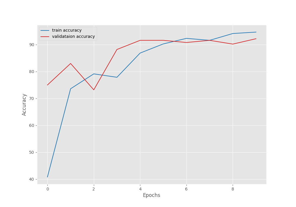
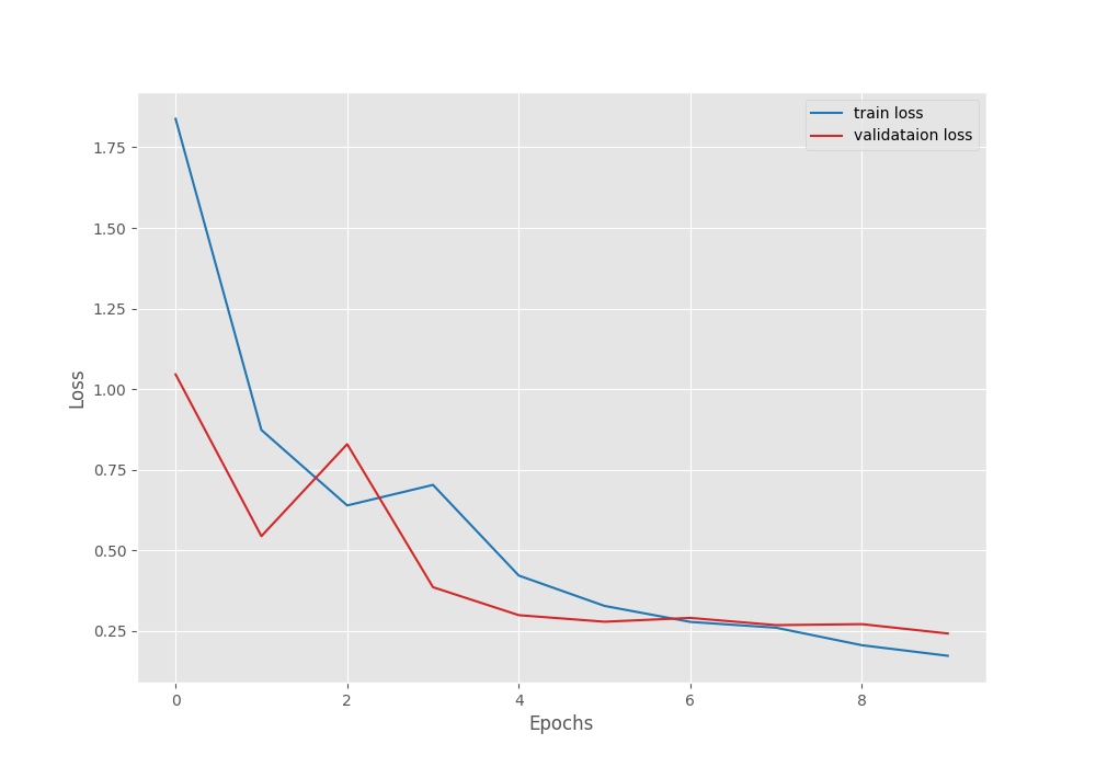
We can see that although on an improving trend, both, the accuracy and loss graphs are fluctuating a bit. If we start with a slightly lower learning rate, we can train even longer to reach a higher accuracy.

For now, we have a trained model with us. Let’s move on to the inference phase.

Inference using the Trained Swin Transformer Model

For inference, we have a set of unseen images (one from each class) from the internet. This will give us an overall idea of how well our model has learned the features of the dataset.

All the inference code will go into the inference.py script.

Starting with the imports, defining a few constants, and the argument parser.

import torch
import numpy as np
import cv2
import os
import torch.nn.functional as F
import torchvision.transforms as transforms
import glob
import argparse
import pathlib

from model import build_model

# Construct the argument parser.
parser = argparse.ArgumentParser()
parser.add_argument(
    '-w', '--weights', 
    default='../outputs/best_model.pth',
    help='path to the model weights',
)
args = vars(parser.parse_args())

# Constants and other configurations.
DEVICE = torch.device('cuda:0' if torch.cuda.is_available() else 'cpu')
IMAGE_RESIZE = 224
CLASS_NAMES = ['apple_pie', 'bibimbap', 'cannoli', 'edamame', 'falafel', 'french_toast', 'ice_cream', 'ramen', 'sushi', 'tiramisu']

The argument parser already points to the default path of the model. Other than that, we have defined the computation device, the image size, and the class names from the dataset.

Now, let’s define three necessary helper functions.

# Validation transforms
def get_test_transform(image_size):
    test_transform = transforms.Compose([
        transforms.ToPILImage(),
        transforms.Resize((image_size, image_size)),
        transforms.ToTensor(),
        transforms.Normalize(
            mean=[0.485, 0.456, 0.406],
            std=[0.229, 0.224, 0.225]
            )
    ])
    return test_transform

def annotate_image(output_class, orig_image):
    class_name = CLASS_NAMES[int(output_class)]
    cv2.putText(
        orig_image, 
        f"{class_name}", 
        (5, 35), 
        cv2.FONT_HERSHEY_SIMPLEX, 
        1.5, 
        (0, 0, 255), 
        2, 
        lineType=cv2.LINE_AA
    )
    return orig_image

def inference(model, testloader, device, orig_image):
    """
    Function to run inference.

    :param model: The trained model.
    :param testloader: The test data loader.
    :param DEVICE: The computation device.
    """
    model.eval()
    counter = 0
    with torch.no_grad():
        counter += 1
        image = testloader
        image = image.to(device)

        # Forward pass.
        outputs = model(image)
    # Softmax probabilities.
    predictions = F.softmax(outputs, dim=1).cpu().numpy()
    # Predicted class number.
    output_class = np.argmax(predictions)
    # Show and save the results.
    result = annotate_image(output_class, orig_image)
    return result

The get_test_transform function defines image transforms that are the same as the one used in the validation data loader while training the model. Further, we have the inference function which accepts the trained Swin Transformer model, the image tensor (testloader), the computation device, and the original image as well. It carries out the forward pass and calls the annotate_image function to annotate the predicted class name string on top of the image.

Finally, the main code block.

if __name__ == '__main__':
    weights_path = pathlib.Path(args['weights'])
    infer_result_path = os.path.join(
        '..', 'outputs', 'inference_results'
    )
    os.makedirs(infer_result_path, exist_ok=True)

    checkpoint = torch.load(weights_path)
    # Load the model.
    model = build_model(
        fine_tune=False, 
        num_classes=len(CLASS_NAMES)
    ).to(DEVICE)
    model.load_state_dict(checkpoint['model_state_dict'])

    all_image_paths = glob.glob(os.path.join('..', 'input', 'inference_data', '*'))

    transform = get_test_transform(IMAGE_RESIZE)

    for i, image_path in enumerate(all_image_paths):
        print(f"Inference on image: {i+1}")
        image = cv2.imread(image_path)
        orig_image = image.copy()
        image = cv2.cvtColor(image, cv2.COLOR_BGR2RGB)
        image = transform(image)
        image = torch.unsqueeze(image, 0)
        result = inference(
            model, 
            image,
            DEVICE,
            orig_image
        )
        # Save the image to disk.
        image_name = image_path.split(os.path.sep)[-1]
        cv2.imshow('Image', result)
        cv2.waitKey(1)
        cv2.imwrite(
            os.path.join(infer_result_path, image_name), result
        )

Here, we simply load the model weights, read all the images from the inference data directory, convert the images to tensor, and carry out inference.

In the end, we show the image on the screen and save the results to outputs/inference_results directory.

Executing the Inference Script

We can execute the following command to start the inference.

python inference.py

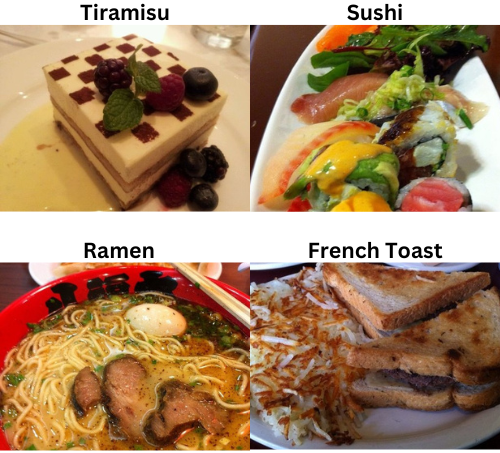
Here are the results.

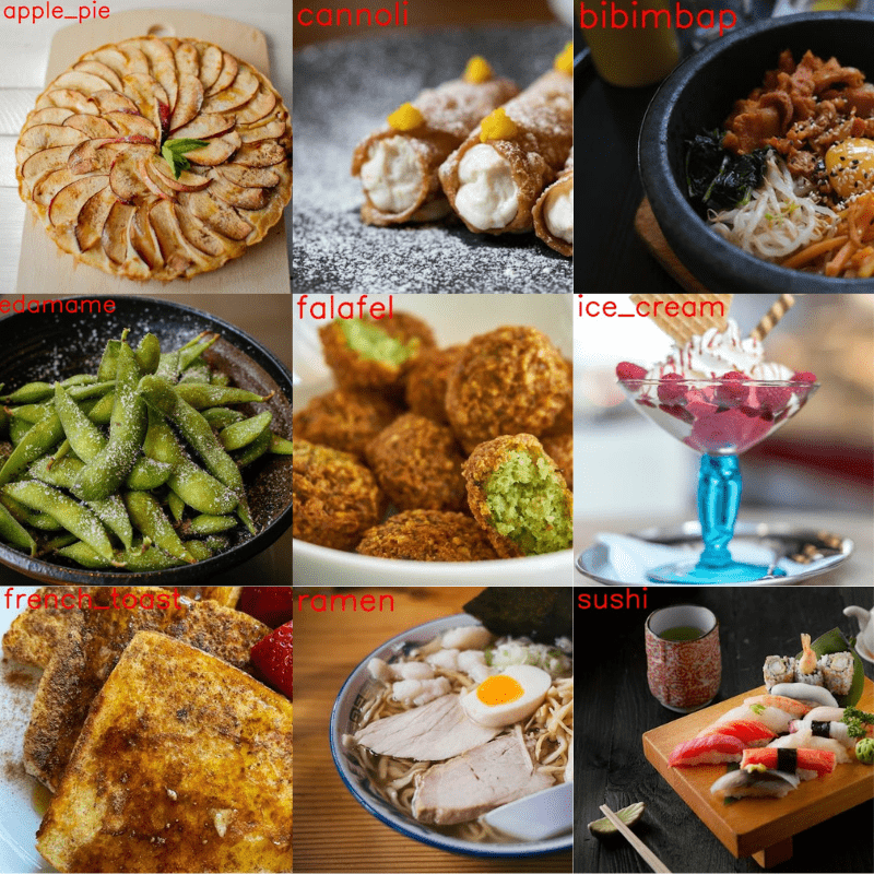
Surprisingly, the Swin Transformer Tiny model predicts all the image classes correctly. Even being a small model and with just 150 training images per class, Swin Transformer is doing extremely well on this image classification task.

Summary and Conclusion

In this blog post, we carried out image classification on the Food-101 Tiny dataset using the Swin Transformer Tiny model. Starting from the dataset preparation to the inference using the trained model, we covered all the parts. This is a tiny glimpse of getting started with Swin Transformer in Computer Vision. In future posts, we will cover more advanced topics using Swin Transformer, like object detection, image segmentation, and image restoration. I hope that this article was worth your time.

If you have any doubts, thoughts, or suggestions, please leave them in the comment section. I will surely address them.

You can contact me using the Contact section. You can also find me on LinkedIn, and Twitter.