Training SegFormer for Person Segmentation

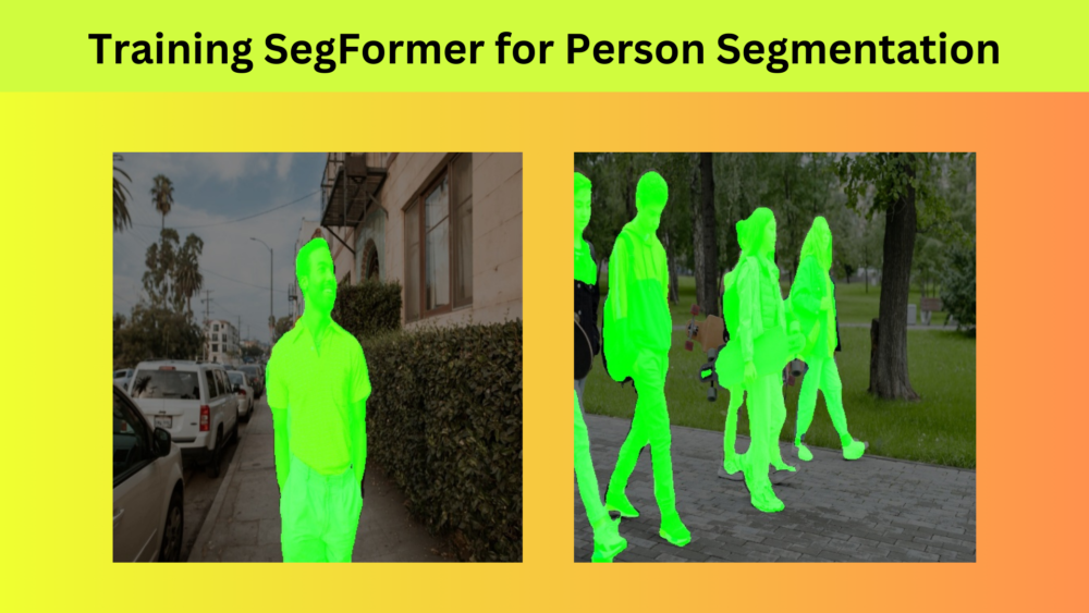
SegFormer is a Transformer based semantic segmentation model. In the last blog post, we went through the summary of SegFormer. Along with that, we also carried out image and video inference using pretrained SegFormer models. In this blog post, we will start with training SegFormer on a custom dataset. We will be training the SegFormer on a person segmentation dataset. This will be a starting point for understanding the entire pipeline of training SegFormer on our own datasets.

Person segmentation in videos is one of the most important practical problems in computer vision. One use case is background blurring in video calls and meets where accurate person segmentation is required in real time. Although, we will not be trying to build such an application here, we can at least get started with using SegFormer for Person Segmentaion on a very small dataset.

What will we cover in this blog post?

• We will start with the discussion of the person segmentation dataset. For training the SegFormer model, we will use the Penn-Fudan Pedestrian segmentation dataset.
• Next, we will move to the coding section. Here, we will discuss each Python file in as much detail as necessary. Mostly, we will focus on preparing the model and the training and validation scripts.
• After training, we will carry out inference on images and videos. This will give us an idea of how well our model works in real world scenarios for person segmentation.

The Penn-Fudan Pedestrian Segmentation Dataset

The Penn-Fudan Pedestrian segmentation dataset contains images and segmented masks of pedestrians. It is perfect to try out training a new segmentation model. This is because it contains just 146 training samples and 24 validation samples.

You can find the dataset here on Kaggle. The following are some of the images and corresponding masks from the dataset.

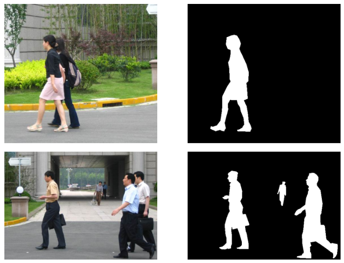
As we can see, the segmentation instances are in various poses and angles. This will help the model learn the segmentation masks in varying scenarios. However, the small size of the dataset may cause issues with learning as Transformer based models generally need large datasets. SegFormer is no exception in this case.

After downloading and extracting the dataset, you should see the following structure.

PennFudanPed/
├── train_images
├── train_masks
├── valid_images
└── valid_masks

The dataset gets extracted into the PennFudanPed directory. The train and validation datasets are present in their respective directories.

One thing to note about the dataset is the segmentation mask format. All the masks are in grayscale. Every person has a segmentation mask with a different pixel value. So, if there are two persons in the same image, then the pixel values of the first will be 1 and the second person will be 2. We will handle this in the dataset preparation part.

Project Directory Structure

Let’s take a look at the entire project directory structure before training the SegFormer model for Person Segmentation.

├── input
│   ├── inference_data
│   ├── PennFudanPed
│   └── penn-fudan-pedestrian-dataset-for-segmentation.zip
├── outputs
│   ├── final_model
│   ├── inference_results_video
│   ├── model_iou
│   ├── model_loss
│   ├── valid_preds
│   ├── accuracy.png
│   ├── loss.png
│   └── miou.png
├── config.py
├── datasets.py
├── engine.py
├── infer_image.py
├── infer_video.py
├── metrics.py
├── model.py
├── train.py
└── utils.py

• The input directory contains the training and inference data. PennFudanPed subdirectory contains the person segmentation dataset that we saw in the previous section. The inference_data subdirectory contains images and videos for inference that we will use after training the SegFormer model.
• The outputs directory will contain all the outputs from the training and inference. These include the trained models, the generated plots, and results from image & video inference.
• Directly inside the project directory, we have the Python files. We will discuss all the essential scripts as we move along the coding section.

The Python files and trained weights will be provided through the download section. In case you don’t want to run training, you can directly run inference using the trained weights.

Installing Dependencies

Before we move forward with the coding section, we need to install the necessary dependencies that we need to train SegFormer. It is best to use an Anaconda environment.

First and foremost, we need to install PyTorch with CUDA support.

conda install pytorch torchvision torchaudio pytorch-cuda=11.7 -c pytorch -c nvidia

The rest of the packages are from Hugging Face. We will use the Hugging Face Transfomers library for loading the SegFormer model.

pip install transformers
pip install evaluate
pip install accelerate -U 

The final important package is Albumentations for image augmentation.

pip install -U albumentations --no-binary qudida,albumentations

You may need other minor packages which you can install on a need basis as you move forward with the code.

Training SegFormer

From here onward, we will start discussing the coding part of the blog post in detail.

Download Code

The Configuration File

We will start with defining the configuration file. This file contains the class names, the label colors for data preparation, and the label color for visualization. This goes into the config.py file.

ALL_CLASSES = ['background', 'person']

LABEL_COLORS_LIST = [
    (0, 0, 0), # Background.
    (255, 255, 255),
]

VIS_LABEL_MAP = [
    (0, 0, 0), # Background.
    (0, 255, 0),
]

The ALL_CLASSES list contains the class names. Although we do not necessarily need the class names, it is good to have the information defined somewhere. In our case, the Penn-Fudan pedestrian segmentation dataset contains just two classes, background and the person class.

Next, we have the LABEL_COLORS_LIST. This defines the color palette for the background and person class that we will use while preparing the dataset. We will define all the pixel values of the background as black, and all that of persons as white.

The VIS_LABEL_MAP lists the color of the pixels that we will use for visualization. During visualization, we will use the green color instead of white for annotating the persons.

Utility Functions and Classes

Next, we need to define some helper functions and classes. All of these will remain in the utils.py file.

Let’s start with importing all the required modules and packages.

import numpy as np
import cv2
import torch
import os
import matplotlib.pyplot as plt
import torch.nn as nn

from config import (
    VIS_LABEL_MAP as viz_map
)

plt.style.use('ggplot')

Note that we import the VIS_LABEL_MAP list from the configuration file. We will discuss its necessity later on.

Functions to Set Class Values

Every object (class) in an image mask will be assigned a different value. For example, in our cases, we have the background and person class. So, the background will have a value of 0 and the person will have a value of 1. We need two functions for that.

def set_class_values(all_classes, classes_to_train):
    """
    This (`class_values`) assigns a specific class label to the each of the classes.
    For example, `animal=0`, `archway=1`, and so on.

    :param all_classes: List containing all class names.
    :param classes_to_train: List containing class names to train.
    """
    class_values = [all_classes.index(cls.lower()) for cls in classes_to_train]
    return class_values

def get_label_mask(mask, class_values, label_colors_list):
    """
    This function encodes the pixels belonging to the same class
    in the image into the same label

    :param mask: NumPy array, segmentation mask.
    :param class_values: List containing class values, e.g car=0, bus=1.
    :param label_colors_list: List containing RGB color value for each class.
    """
    label_mask = np.zeros((mask.shape[0], mask.shape[1]), dtype=np.uint8)
    for value in class_values:
        for ii, label in enumerate(label_colors_list):
            if value == label_colors_list.index(label):
                label = np.array(label)
                label_mask[np.where(np.all(mask == label, axis=-1))[:2]] = value
    label_mask = label_mask.astype(int)
    return label_mask

The set_class_values will set a value starting from 0 to the number of classes – 1 for each class. In case we do not want to train a model on all the classes, we can manage the classes_to_train list accordingly and only pass the class names that we want. It will return a list [0, 1] in our case as we have just the background and person class.

The next function, get_label_mask accepts an RGB mask, the class values from the above function, and a list containing the colors that we want to encode each class’ pixel with. It returns a grayscale mask of the shape height X width.

Visualizing Validation Samples Inbetween Training

During the validation step of each training epoch, we will save an evaluation sample from one batch. This will help us track the progress of the model as we get to see the segmentation ability right away.

The following two functions handle that.

def denormalize(x, mean=None, std=None):
    # x should be a Numpy array of shape [H, W, C] 
    x = torch.tensor(x).permute(2, 0, 1).unsqueeze(0)
    for t, m, s in zip(x, mean, std):
        t.mul_(s).add_(m)
    res = torch.clamp(t, 0, 1)
    res = res.squeeze(0).permute(1, 2, 0).numpy()
    return res

def draw_translucent_seg_maps(
    data, 
    output, 
    epoch, 
    i, 
    val_seg_dir, 
    label_colors_list,
):
    """
    This function color codes the segmentation maps that is generated while
    validating. THIS IS NOT TO BE CALLED FOR SINGLE IMAGE TESTING
    """
    IMG_MEAN = [0.485, 0.456, 0.406]
    IMG_STD = [0.229, 0.224, 0.225]
    alpha = 1 # how much transparency
    beta = 0.8 # alpha + beta should be 1
    gamma = 0 # contrast

    seg_map = output[0] # use only one output from the batch
    seg_map = torch.argmax(seg_map.squeeze(), dim=0).detach().cpu().numpy()

    image = denormalize(data[0].permute(1, 2, 0).cpu().numpy(), IMG_MEAN, IMG_STD)

    red_map = np.zeros_like(seg_map).astype(np.uint8)
    green_map = np.zeros_like(seg_map).astype(np.uint8)
    blue_map = np.zeros_like(seg_map).astype(np.uint8)

    for label_num in range(0, len(label_colors_list)):
        index = seg_map == label_num
        red_map[index] = np.array(viz_map)[label_num, 0]
        green_map[index] = np.array(viz_map)[label_num, 1]
        blue_map[index] = np.array(viz_map)[label_num, 2]
        
    rgb = np.stack([red_map, green_map, blue_map], axis=2)
    rgb = np.array(rgb, dtype=np.float32)
    # convert color to BGR format for OpenCV
    rgb = cv2.cvtColor(rgb, cv2.COLOR_RGB2BGR)
    # cv2.imshow('rgb', rgb)
    # cv2.waitKey(0)
    image = cv2.cvtColor(image, cv2.COLOR_RGB2BGR) * 255.
    cv2.addWeighted(image, alpha, rgb, beta, gamma, image)
    cv2.imwrite(f"{val_seg_dir}/e{epoch}_b{i}.jpg", image)

The draw_translucent_seg_maps function accepts the image batch and the output from the model. Along with that it also accepts a few more information such as the batch number (i), the epoch number, and of course a list of color palettes for visualization.

First, we extract one image from the batch and denormalize it using the denormalize function. Next, we create the RGB segmentation map (rgb). Finally, we overlap the image on the RGB segmentation map and save it to disk.

Saving Models and Graphs

We always want to save the best performing models. The following classes and functions help us achieve that.

class SaveBestModel:
    """
    Class to save the best model while training. If the current epoch's 
    validation loss is less than the previous least less, then save the
    model state.
    """
    def __init__(self, best_valid_loss=float('inf')):
        self.best_valid_loss = best_valid_loss
        
    def __call__(
        self, current_valid_loss, epoch, model, out_dir, name='model'
    ):
        if current_valid_loss < self.best_valid_loss:
            self.best_valid_loss = current_valid_loss
            print(f"\nBest validation loss: {self.best_valid_loss}")
            print(f"\nSaving best model for epoch: {epoch+1}\n")
            model.save_pretrained(os.path.join(out_dir, name))

class SaveBestModelIOU:
    """
    Class to save the best model while training. If the current epoch's 
    IoU is higher than the previous highest, then save the
    model state.
    """
    def __init__(self, best_iou=float(0)):
        self.best_iou = best_iou
        
    def __call__(self, current_iou, epoch, model, out_dir, name='model'):
        if current_iou > self.best_iou:
            self.best_iou = current_iou
            print(f"\nBest validation IoU: {self.best_iou}")
            print(f"\nSaving best model for epoch: {epoch+1}\n")
            model.save_pretrained(os.path.join(out_dir, name))

def save_model(model, out_dir, name='model'):
    """
    Function to save the trained model to disk.
    """
    model.save_pretrained(os.path.join(out_dir, name))

We save the models according to three criteria:

• According to the least validation loss.
• According to the highest mean IoU score.
• And the final model once the training finishes.

This will give us plenty of options to either run inference or even resume training using the final model.

Note that we use the save_pretrained method of the Hugging Face Transformer model for saving the best models and the final model as well.

Along with the models, we also save the graphs for the loss, the pixel accuracy, and the mean IoU metric.

def save_plots(
    train_acc, valid_acc, 
    train_loss, valid_loss, 
    train_miou, valid_miou, 
    out_dir
):
    """
    Function to save the loss and accuracy plots to disk.
    """
    # Accuracy plots.
    plt.figure(figsize=(10, 7))
    plt.plot(
        train_acc, color='tab:blue', linestyle='-', 
        label='train accuracy'
    )
    plt.plot(
        valid_acc, color='tab:red', linestyle='-', 
        label='validataion accuracy'
    )
    plt.xlabel('Epochs')
    plt.ylabel('Accuracy')
    plt.legend()
    plt.savefig(os.path.join(out_dir, 'accuracy.png'))
    
    # Loss plots.
    plt.figure(figsize=(10, 7))
    plt.plot(
        train_loss, color='tab:blue', linestyle='-', 
        label='train loss'
    )
    plt.plot(
        valid_loss, color='tab:red', linestyle='-', 
        label='validataion loss'
    )
    plt.xlabel('Epochs')
    plt.ylabel('Loss')
    plt.legend()
    plt.savefig(os.path.join(out_dir, 'loss.png'))

    # mIOU plots.
    plt.figure(figsize=(10, 7))
    plt.plot(
        train_miou, color='tab:blue', linestyle='-', 
        label='train mIoU'
    )
    plt.plot(
        valid_miou, color='tab:red', linestyle='-', 
        label='validataion mIoU'
    )
    plt.xlabel('Epochs')
    plt.ylabel('mIoU')
    plt.legend()
    plt.savefig(os.path.join(out_dir, 'miou.png'))

The save_plots function accepts the lists containing the respective values of loss and metrics and saves the graphs to disk.

Helper Functions for Inference

The final three helper functions in utils.py will aid during inference.

def predict(model, extractor, image, device):
    """
    :param model: The Segformer model.
    :param extractor: The Segformer feature extractor.
    :param image: The image in RGB format.
    :param device: The compute device.

    Returns:
        labels: The final labels (classes) in h x w format.
    """
    pixel_values = extractor(image, return_tensors='pt').pixel_values.to(device)
    with torch.no_grad():
        logits = model(pixel_values).logits

    # Rescale logits to original image size.
    logits = nn.functional.interpolate(
        logits,
        size=image.shape[:2],
        mode='bilinear',
        align_corners=False
    )

    # Get class labels.
    labels = torch.argmax(logits.squeeze(), dim=0)

    return labels

def draw_segmentation_map(labels, palette):
    """
    :param labels: Label array from the model.Should be of shape 
        <height x width>. No channel information required.
    :param palette: List containing color information.
        e.g. [[0, 255, 0], [255, 255, 0]] 
    """
    # create Numpy arrays containing zeros
    # later to be used to fill them with respective red, green, and blue pixels
    red_map = np.zeros_like(labels).astype(np.uint8)
    green_map = np.zeros_like(labels).astype(np.uint8)
    blue_map = np.zeros_like(labels).astype(np.uint8)

    for label_num in range(0, len(palette)):
        index = labels == label_num
        red_map[index] = np.array(palette)[label_num, 0]
        green_map[index] = np.array(palette)[label_num, 1]
        blue_map[index] = np.array(palette)[label_num, 2]
        
    segmentation_map = np.stack([red_map, green_map, blue_map], axis=2)
    return segmentation_map

def image_overlay(image, segmented_image):
    """
    :param image: Image in RGB format.
    :param segmented_image: Segmentation map in RGB format. 
    """
    alpha = 0.5 # transparency for the original image
    beta = 1.0 # transparency for the segmentation map
    gamma = 0 # scalar added to each sum

    segmented_image = cv2.cvtColor(segmented_image, cv2.COLOR_RGB2BGR)
    image = np.array(image)
    image = cv2.cvtColor(image, cv2.COLOR_RGB2BGR)
    cv2.addWeighted(image, alpha, segmented_image, beta, gamma, image)
    return image

The predict function essentially carries out the forward pass of the image through the model. You can go through the previous post where use SegFormer for inference to get a detailed view of the function.

The draw_segmentation_map function creates the RGB segmentation map from the model output and returns it. The final function, that is, image_overlay overlays the original image on the RGB segmentation map.

This brings us to the end of all the utilities that we need along the way.

Metrics for Evaluating the Performance of SegFormer

Our primary evaluation metric is going to be mIoU (Mean Intersection Over Union). It is one of the most commonly used metrics even for pretraining semantic segmentation models.

The code for mIoU will go into the metrics.py file.

import numpy as np

# Source: https://github.com/sacmehta/ESPNet/blob/master/train/IOUEval.py

class IOUEval:
    def __init__(self, nClasses):
        self.nClasses = nClasses
        self.reset()

    def reset(self):
        self.overall_acc = 0
        self.per_class_acc = np.zeros(self.nClasses, dtype=np.float32)
        self.per_class_iu = np.zeros(self.nClasses, dtype=np.float32)
        self.mIOU = 0
        self.batchCount = 1

    def fast_hist(self, a, b):
        k = (a >= 0) & (a < self.nClasses)
        return np.bincount(self.nClasses * a[k].astype(int) + b[k], minlength=self.nClasses ** 2).reshape(self.nClasses, self.nClasses)

    def compute_hist(self, predict, gth):
        hist = self.fast_hist(gth, predict)
        return hist

    def addBatch(self, predict, gth):
        predict = predict.cpu().numpy().flatten()
        gth = gth.cpu().numpy().flatten()

        epsilon = 0.00000001
        hist = self.compute_hist(predict, gth)
        overall_acc = np.diag(hist).sum() / (hist.sum() + epsilon)
        per_class_acc = np.diag(hist) / (hist.sum(1) + epsilon)
        per_class_iu = np.diag(hist) / (hist.sum(1) + hist.sum(0) - np.diag(hist) + epsilon)
        mIou = np.nanmean(per_class_iu)

        self.overall_acc +=overall_acc
        self.per_class_acc += per_class_acc
        self.per_class_iu += per_class_iu
        self.mIOU += mIou
        self.batchCount += 1

    def getMetric(self):
        overall_acc = self.overall_acc/self.batchCount
        per_class_acc = self.per_class_acc / self.batchCount
        per_class_iu = self.per_class_iu / self.batchCount
        mIOU = self.mIOU / self.batchCount

        return overall_acc, per_class_acc, per_class_iu, mIOU

The code for the above IOUEval class has been borrowed from the ESPNet segmentation model repository. Although, we will also measure the pixel accuracy of the mode, mIoU is going to be our primary evaluation metric while training the SegFormer model.

Preparing the Person Segmentation Dataset

Preparing semantic segmentation datasets is not always very straightforward. Sometimes we need to handle a few edge cases manually so that the dataset preparation goes smoothly.

Let’s go through the datasets.py file which contains the code for preparing the datasets and data loaders.

Defining Data Paths and Transforms

We will start with the imports and defining functions for data paths and transforms.

import glob
import albumentations as A
import cv2
import numpy as np

from utils import get_label_mask, set_class_values
from torch.utils.data import Dataset, DataLoader
from PIL import Image

def get_images(root_path):
    train_images = glob.glob(f"{root_path}/train_images/*")
    train_images.sort()
    train_masks = glob.glob(f"{root_path}/train_masks/*")
    train_masks.sort()
    valid_images = glob.glob(f"{root_path}/valid_images/*")
    valid_images.sort()
    valid_masks = glob.glob(f"{root_path}/valid_masks/*")
    valid_masks.sort()

    return train_images, train_masks, valid_images, valid_masks

def train_transforms(img_size):
    """
    Transforms/augmentations for training images and masks.

    :param img_size: Integer, for image resize.
    """
    train_image_transform = A.Compose([
        A.Resize(img_size[1], img_size[0], always_apply=True),
        A.HorizontalFlip(p=0.5),
        A.RandomBrightnessContrast(p=0.2),
        A.Rotate(limit=25)
    ])
    return train_image_transform

def valid_transforms(img_size):
    """
    Transforms/augmentations for validation images and masks.

    :param img_size: Integer, for image resize.
    """
    valid_image_transform = A.Compose([
        A.Resize(img_size[1], img_size[0], always_apply=True),
    ])
    return valid_image_transform

We are importing the get_label_mask and set_class_values functions from the utils module as we need them later on.

The get_images function captures all the images and corresponding mask paths and sorts them in a list. It ensures that each index of an image list should have a corresponding segmentation mask path in the mask list.

The train_transforms applies the necessary transforms to images and masks. It resizes and augments the images. However, as we are using Albumetations, it ensures that pixel-level augmentations like brightness and contrast are not applied to the masks.

The valid_transforms is for the validation dataset and it just resizes the images and masks.

The Custom Segmentation Dataset Class

We need to define a custom dataset class to get the data in the desired format. The following code block defines a SegmentationDataset class.

class SegmentationDataset(Dataset):
    def __init__(
        self, 
        image_paths, 
        mask_paths, 
        tfms, 
        label_colors_list,
        classes_to_train,
        all_classes,
        feature_extractor
    ):
        self.image_paths = image_paths
        self.mask_paths = mask_paths
        self.tfms = tfms
        self.label_colors_list = label_colors_list
        self.all_classes = all_classes
        self.classes_to_train = classes_to_train
        self.class_values = set_class_values(
            self.all_classes, self.classes_to_train
        )
        self.feature_extractor = feature_extractor

    def __len__(self):
        return len(self.image_paths)

    def __getitem__(self, index):
        image = cv2.imread(self.image_paths[index], cv2.IMREAD_COLOR)
        image = cv2.cvtColor(image, cv2.COLOR_BGR2RGB).astype('float32')
        mask = cv2.imread(self.mask_paths[index], cv2.IMREAD_COLOR)
        mask = cv2.cvtColor(mask, cv2.COLOR_BGR2RGB).astype('float32')

        # Make all pixel > 0 as 255.
        im = mask > 0
        mask[im] = 255
        mask[np.logical_not(im)] = 0

        transformed = self.tfms(image=image, mask=mask)
        image = transformed['image'].astype('uint8')
        mask = transformed['mask']
        
        # Get 2D label mask.
        mask = get_label_mask(mask, self.class_values, self.label_colors_list).astype('uint8')
        mask = Image.fromarray(mask)
               
        encoded_inputs = self.feature_extractor(
            Image.fromarray(image), 
            mask,
            return_tensors='pt'
        )
        for k, v in encoded_inputs.items():
            encoded_inputs[k].squeeze_()

        return encoded_inputs

We pass the following parameters while initializing the SegmentationDataset class.

• image_paths and mask_paths: The list containing the image and mask paths that we get from the get_images function.
• tfms: This represents the transforms that we want to apply. We have defined the transforms in the previous code block.
• label_colors_list: This is a list containing the color values for each class.
• classes_to_train and all_classes: These are lists containing the string names of classes that we want to train and all the class names in the dataset.
• feature_extractor: The Transformers library provides a feature extractor class for the SegFormer model. This helps us apply the necessary ImageNet normalization.

There are a few important points to note in the __getitem__ method.

• We read the mask as an RGB image and convert all the pixel values that are greater than 1 to 255. You may remember that each person in the dataset has a different pixel value. As we want to do semantic segmentation here, we just convert each person’s pixel values to 255 (lines 78 to 80).
• Then we apply the transforms to the images and masks using Albumentations.
• On line 87, we get the 2D label mask of the shape height X width.
• Next, we use the SegFormer feature extractor to get the encoded pixel values on line 90. It returns PyTorch tensors as we provide return_tensors='pt'.
• Finally, we remove the batch dimensions from the encoded inputs and return them.

Functions to Create Datasets and Data Loaders

The final part of the dataset preparation includes defining the functions to create the datasets and data loaders.

def get_dataset(
    train_image_paths, 
    train_mask_paths,
    valid_image_paths,
    valid_mask_paths,
    all_classes,
    classes_to_train,
    label_colors_list,
    img_size,
    feature_extractor
):
    train_tfms = train_transforms(img_size)
    valid_tfms = valid_transforms(img_size)

    train_dataset = SegmentationDataset(
        train_image_paths,
        train_mask_paths,
        train_tfms,
        label_colors_list,
        classes_to_train,
        all_classes, 
        feature_extractor
    )
    valid_dataset = SegmentationDataset(
        valid_image_paths,
        valid_mask_paths,
        valid_tfms,
        label_colors_list,
        classes_to_train,
        all_classes,
        feature_extractor
    )
    return train_dataset, valid_dataset

def get_data_loaders(train_dataset, valid_dataset, batch_size):
    train_data_loader = DataLoader(
        train_dataset, 
        batch_size=batch_size, 
        drop_last=False, 
        num_workers=8,
        shuffle=True
    )
    valid_data_loader = DataLoader(
        valid_dataset, 
        batch_size=batch_size, 
        drop_last=False, 
        num_workers=8,
        shuffle=False
    )

    return train_data_loader, valid_data_loader

The get_datasets function creates the training and validation datasets by initializing the SegmentationDataset class with the necessary arguments.

The get_data_loaders function creates the respective data loaders. We use 8 parallel workers for data loading. You can use more if your system has a higher number of logical cores.

This concludes the code needed for dataset preparation.

The Training and Validation Functions

We need to define the training and validation functions for carrying out training of the SegFormer model.

The engine.py file holds the code for this.

First, we have the import statements.

import torch
import torch.nn as nn

from tqdm import tqdm
from utils import draw_translucent_seg_maps
from metrics import IOUEval

We are importing the draw_translucent_seg_maps function from utils to draw the predicted segmentation map of one image during validation. The IoUEval class is for calculating the mIoU metric.

The SegFormer Training Function

def train(
    model,
    train_dataloader,
    device,
    optimizer,
    classes_to_train
):
    print('Training')
    model.train()
    train_running_loss = 0.0
    prog_bar = tqdm(
        train_dataloader, 
        total=len(train_dataloader), 
        bar_format='{l_bar}{bar:20}{r_bar}{bar:-20b}'
    )
    counter = 0 # to keep track of batch counter
    num_classes = len(classes_to_train)
    iou_eval = IOUEval(num_classes)

    for i, data in enumerate(prog_bar):
        counter += 1
        pixel_values, target = data['pixel_values'].to(device), data['labels'].to(device)
        optimizer.zero_grad()
        outputs = model(pixel_values=pixel_values, labels=target)

        ##### BATCH-WISE LOSS #####
        loss = outputs.loss
        train_running_loss += loss.item()
        ###########################

        ##### BACKPROPAGATION AND PARAMETER UPDATION #####
        loss.backward()
        optimizer.step()
        ##################################################

        logits = outputs.logits
        upsampled_logits = nn.functional.interpolate(
            logits, size=target.shape[-2:], 
            mode="bilinear", 
            align_corners=False
        )
        iou_eval.addBatch(upsampled_logits.max(1)[1].data, target.data)
        
    ##### PER EPOCH LOSS #####
    train_loss = train_running_loss / counter
    ##########################
    overall_acc, per_class_acc, per_class_iou, mIOU = iou_eval.getMetric()
    return train_loss, overall_acc, mIOU

The train function accepts the model, training data loader, computation device, optimizer, and the list of classes to train as parameters.

When iterating through the data loader, we carry out the following steps:

• Each batch contains a dictionary. The pixel_values key holds the processed image and the labels key holds the segmentation map. We extract these first.
• When forward passing the data through the model, we need to pass both, the image pixel values and the target segmentation map.
• The outputs that we get holds the model’s logits and loss in their respective keys. The output is a dictionary. We do not need our own loss function in this case.
• The logits are downsampled ones from the final layer of the SegFormer MLP decoder. We upsample the logits using PyTorch’s nn.functional.interpolate to resize them to the same size as the target segmentation map. Then we pass this to the addBatch method of the iou_eval instance to calculate the per batch pixel accuracy and mIOU.
• Along with that, we do the mandatory backward propagation and updating the model weights using the optimizer.

The SegFormer Validation Function

def validate(
    model,
    valid_dataloader,
    device,
    classes_to_train,
    label_colors_list,
    epoch,
    save_dir
):
    print('Validating')
    model.eval()
    valid_running_loss = 0.0
    num_classes = len(classes_to_train)
    iou_eval = IOUEval(num_classes)

    with torch.no_grad():
        prog_bar = tqdm(
            valid_dataloader, 
            total=(len(valid_dataloader)), 
            bar_format='{l_bar}{bar:20}{r_bar}{bar:-20b}'
        )
        counter = 0 # To keep track of batch counter.
        for i, data in enumerate(prog_bar):
            counter += 1
            pixel_values, target = data['pixel_values'].to(device), data['labels'].to(device)
            outputs = model(pixel_values=pixel_values, labels=target)

            logits = outputs.logits
            upsampled_logits = nn.functional.interpolate(
                logits, size=target.shape[-2:], 
                mode="bilinear", 
                align_corners=False
            )
            
            # Save the validation segmentation maps.
            if i == 1:
                draw_translucent_seg_maps(
                    pixel_values, 
                    upsampled_logits, 
                    epoch, 
                    i, 
                    save_dir, 
                    label_colors_list,
                )

            ##### BATCH-WISE LOSS #####
            loss = outputs.loss
            valid_running_loss += loss.item()
            ###########################

            iou_eval.addBatch(upsampled_logits.max(1)[1].data, target.data)
        
    ##### PER EPOCH LOSS #####
    valid_loss = valid_running_loss / counter
    ##########################
    overall_acc, per_class_acc, per_class_iou, mIOU = iou_eval.getMetric()
    return valid_loss, overall_acc, mIOU

The validation loop is similar to the training one except we do not need to update any optimizer state or backpropagation.

Furthermore, we call the draw_translucent_seg_maps to save one image along with its predicted segmentation map to disk.

Just like the training loop, here also, we return the validation loss, the pixel accuracy, and the validation mIoU.

The SegFormer-B1 Model

As discussed earlier, we use the SegFormer model from the Transformers library. We will not be using any fine-tuned model. Instead, we will build the SegFormer model using the MiT-B1 encoder which has been pretrained on the ImageNet-1K dataset.

The code for this remains in the model.py file.

from transformers import SegformerForSemanticSegmentation

def segformer_model(classes):
    model = SegformerForSemanticSegmentation.from_pretrained(
        'nvidia/mit-b1',
        num_labels=len(classes),
    )
    return model

We import the SegformerForSemanticSegmentation class from the transformers library to build the model. The segformer_model function accepts the classes list using which we feed the information about the number of classes to the from_pretrained method.

The from_pretrained method expects a model name or path. In this case, we provide the Hugging Face repository name where the model is present. The num_labels argument expects the number of classes in our dataset. We have just two classes in our dataset including the background class. The following is the snippet from the model architecture for the final few layers.

(linear_fuse): Conv2d(1024, 256, kernel_size=(1, 1), stride=(1, 1), bias=False)
(batch_norm): BatchNorm2d(256, eps=1e-05, momentum=0.1, affine=True, track_running_stats=True)
(activation): ReLU()
(dropout): Dropout(p=0.1, inplace=False)
(classifier): Conv2d(256, 2, kernel_size=(1, 1), stride=(1, 1))

The final model (SegFormer-B1) roughly contains 13.6 million trainable parameters.

The Training Script

We have reached the training script which is the final Python file before we begin the training. This file connects all the components that we have defined till now.

The code for the training script goes into the train.py file.

Starting with the imports, defining the seed for reproducibility, and the argument parsers.

import torch
import os
import argparse

from datasets import get_images, get_dataset, get_data_loaders
from model import segformer_model
from config import ALL_CLASSES, LABEL_COLORS_LIST
from transformers import SegformerFeatureExtractor
from engine import train, validate
from utils import save_model, SaveBestModel, save_plots, SaveBestModelIOU
from torch.optim.lr_scheduler import MultiStepLR

seed = 42
torch.manual_seed(seed)
torch.cuda.manual_seed(seed)
torch.backends.cudnn.deterministic = True
torch.backends.cudnn.benchmark = True

parser = argparse.ArgumentParser()
parser.add_argument(
    '--epochs',
    default=10,
    help='number of epochs to train for',
    type=int
)
parser.add_argument(
    '--lr',
    default=0.0001,
    help='learning rate for optimizer',
    type=float
)
parser.add_argument(
    '--batch',
    default=4,
    help='batch size for data loader',
    type=int
)
parser.add_argument(
    '--imgsz', 
    default=[512, 416],
    type=int,
    nargs='+',
    help='width, height'
)
parser.add_argument(
    '--scheduler',
    action='store_true',
)
args = parser.parse_args()
print(args)

We can pass values to the following command line arguments:

• --epochs: The number of epochs we want to train the model for.
• --lr: The base learning rate of the optimizer.
• --batch: Batch size for the data loaders.
• --imgsz: The training image size. It accepts multiple arguments for width and height respectively.
• --scheduler: It is a boolean argument indicating whether we want to apply a learning rate scheduler or not. We will define the Multi Step Learning Rate scheduler later in the script.

The Main Code Block

We will define all the training related code inside the main block. The following code block contains the entire for that. It is quite long but is much easier to maintain as we can ensure that nothing gets executed unexpectedly.

if __name__ == '__main__':
    # Create a directory with the model name for outputs.
    out_dir = os.path.join('outputs')
    out_dir_valid_preds = os.path.join('outputs', 'valid_preds')
    os.makedirs(out_dir, exist_ok=True)
    os.makedirs(out_dir_valid_preds, exist_ok=True)

    device = torch.device('cuda:0' if torch.cuda.is_available() else 'cpu')
    model = segformer_model(classes=ALL_CLASSES).to(device)
    print(model)
    # Total parameters and trainable parameters.
    total_params = sum(p.numel() for p in model.parameters())
    print(f"{total_params:,} total parameters.")
    total_trainable_params = sum(
        p.numel() for p in model.parameters() if p.requires_grad)
    print(f"{total_trainable_params:,} training parameters.")

    optimizer = torch.optim.AdamW(model.parameters(), lr=args.lr)

    train_images, train_masks, valid_images, valid_masks = get_images(
        root_path='input/PennFudanPed'    
    )

    feature_extractor = SegformerFeatureExtractor(size=args.imgsz)

    train_dataset, valid_dataset = get_dataset(
        train_images, 
        train_masks,
        valid_images,
        valid_masks,
        ALL_CLASSES,
        ALL_CLASSES,
        LABEL_COLORS_LIST,
        img_size=args.imgsz,
        feature_extractor=feature_extractor
    )

    train_dataloader, valid_dataloader = get_data_loaders(
        train_dataset, 
        valid_dataset,
        args.batch
    )

    # Initialize `SaveBestModel` class.
    save_best_model = SaveBestModel()
    save_best_iou = SaveBestModelIOU()
    # LR Scheduler.
    scheduler = MultiStepLR(
        optimizer, milestones=[30], gamma=0.1, verbose=True
    )

    train_loss, train_pix_acc, train_miou = [], [], []
    valid_loss, valid_pix_acc, valid_miou = [], [], []
    
    for epoch in range (args.epochs):
        print(f"EPOCH: {epoch + 1}")
        train_epoch_loss, train_epoch_pixacc, train_epoch_miou = train(
            model,
            train_dataloader,
            device,
            optimizer,
            ALL_CLASSES
        )
        valid_epoch_loss, valid_epoch_pixacc, valid_epoch_miou = validate(
            model,
            valid_dataloader,
            device,
            ALL_CLASSES,
            LABEL_COLORS_LIST,
            epoch,
            save_dir=out_dir_valid_preds
        )
        train_loss.append(train_epoch_loss)
        train_pix_acc.append(train_epoch_pixacc)
        train_miou.append(train_epoch_miou)
        valid_loss.append(valid_epoch_loss)
        valid_pix_acc.append(valid_epoch_pixacc)
        valid_miou.append(valid_epoch_miou)

        save_best_model(
            valid_epoch_loss, epoch, model, out_dir, name='model_loss'
        )
        save_best_iou(
            valid_epoch_miou, epoch, model, out_dir, name='model_iou'
        )

        print(
            f"Train Epoch Loss: {train_epoch_loss:.4f},",
            f"Train Epoch PixAcc: {train_epoch_pixacc:.4f},",
            f"Train Epoch mIOU: {train_epoch_miou:4f}"
        )
        print(
            f"Valid Epoch Loss: {valid_epoch_loss:.4f},", 
            f"Valid Epoch PixAcc: {valid_epoch_pixacc:.4f}",
            f"Valid Epoch mIOU: {valid_epoch_miou:4f}"
        )
        if args.scheduler:
            scheduler.step()
        print('-' * 50)

    # Save the loss and accuracy plots.
    save_plots(
        train_pix_acc, valid_pix_acc, 
        train_loss, valid_loss,
        train_miou, valid_miou, 
        out_dir
    )
    # Save final model.
    save_model(model, out_dir, name='final_model')
    print('TRAINING COMPLETE')

Let’s go through the code in a step-wise manner.

• First, we define the output directories to save the models and the predictions from the validation loop.
• Next, we define the computation device, the SegFormer-B1 model, and the optimizer. We use the AdamW optimizer which is the same optimizer that was used for fine-tuning on various datasets by the authors. The initial learning rate is 0.0001.
• Then we get the paths to the training images & masks and initialize the SegFormerFeatureExtractor. This will normalize the images and masks with ImageNet statistics. Do note that we pass the image size to the class so that the feature scaling will happen accordingly.
• After that, we initialize the datasets and data loaders. This is followed by initializing the classes to save the best model according to IoU and validation loss. We also initialize the MultiStepLR which will reduce the learning rate by a factor of 10 after 30 epochs. Before starting the training loop, we define the necessary empty lists to store the values for loss, pixel accuracy, and mIoU.
• During the training process, we save the model to disk whenever the current mIoU is better than the previous one and also when the current validation loss is lower than than previous one.
• Finally, we save the graphs to disk and save the model one final time as well.

This covers all the code that we need to start the training of the SegFormer-B1 model for person segmentation.

Executing train.py

We can execute train.py from the parent project directory. To start the training, run the following command.

python train.py --imgsz 512 512 --batch 8 --lr 0.0001 --epochs 60 --scheduler

We are training with an image size of 512×512, batch size of 8, and a base learning rate of 0.0001. The model will train for a total of 60 epochs and the scheduler will be applied after 30 epochs.

Here are the terminal outputs from the final few epochs.

--------------------------------------------------
EPOCH: 49
Training
100%|████████████████████| 19/19 [00:48<00:00,  2.55s/it]                                                                                                                                                          
Validating
100%|████████████████████| 3/3 [00:01<00:00,  1.64it/s]                                                                                                                                                            

Best validation loss: 0.0670458289484183

Saving best model for epoch: 49


Best validation IoU: 0.6866318328981496

Saving best model for epoch: 49

Train Epoch Loss: 0.1154, Train Epoch PixAcc: 0.9064, Train Epoch mIOU: 0.803854
Valid Epoch Loss: 0.0670, Valid Epoch PixAcc: 0.7310 Valid Epoch mIOU: 0.686632
Adjusting learning rate of group 0 to 1.0000e-05.
.
.
.
EPOCH: 59
Training
100%|████████████████████| 19/19 [00:44<00:00,  2.35s/it]                                                                                                                                                          
Validating
100%|████████████████████| 3/3 [00:02<00:00,  1.11it/s]                                                                                                                                                            
Train Epoch Loss: 0.1118, Train Epoch PixAcc: 0.9058, Train Epoch mIOU: 0.810594
Valid Epoch Loss: 0.0676, Valid Epoch PixAcc: 0.7308 Valid Epoch mIOU: 0.685953
Adjusting learning rate of group 0 to 1.0000e-05.
--------------------------------------------------
EPOCH: 60
Training
100%|████████████████████| 19/19 [00:44<00:00,  2.33s/it]                                                                                                                                                          
Validating
100%|████████████████████| 3/3 [00:02<00:00,  1.26it/s]                                                                                                                                                            

Best validation loss: 0.06637159859140714

Saving best model for epoch: 60

Train Epoch Loss: 0.1188, Train Epoch PixAcc: 0.9064, Train Epoch mIOU: 0.806931
Valid Epoch Loss: 0.0664, Valid Epoch PixAcc: 0.7309 Valid Epoch mIOU: 0.686216
Adjusting learning rate of group 0 to 1.0000e-05.
--------------------------------------------------
TRAINING COMPLETE

The best model according to the validation IoU was last saved on epoch 49. It is quite interesting that the validation loss was decreasing till the end of training. However, we will use the model according to the best validation IoU was 68.66.

The following are the graphs for the loss, pixel accuracy, and mIoU.

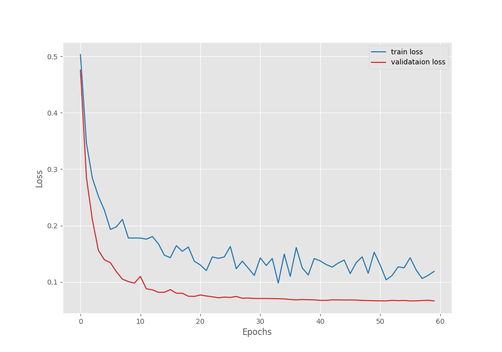
We can see that the validation loss was decreasing till 60 epochs just as we confirmed from the terminal outputs.

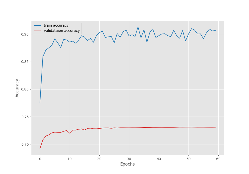
The pixel accuracy almost stagnated after 30 epochs.

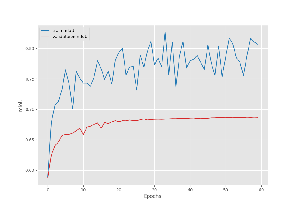
The mIoU plot seems to be plateaued out after epoch 50. It is possible that if we apply a few more augmentations, then we can train for longer and even the mIoU may increase.

We are done with the training part for now. In the next section, we will use the trained SegFormer-B1 model for image and video inference.

Inference using the Trained SegFormer-B1 Model

We have two different scripts for running inference on images and videos. We will not go into the details of these scripts as they are almost the same as in the previous blog post where we ran inference. Please go through the previous post in case you want to know the inference steps in detail.

We will use the model saved with the best mIoU to run inference. Following is the syntax to load the Transformers SegFormer trained weights.

extractor = SegformerFeatureExtractor()
model = SegformerForSemanticSegmentation.from_pretrained('outputs/model_iou')

This time, we do not need to provide any arguments to the SegformerFeatureExtractor. When loading the weights we can use the from_pretrained method and just point to the directory where the trained model is saved. It looks for a JSON file which contains the architecture configuration and a binary model file which contains the weights.

Inference on Images using the Trained SegFormer-B1 Model

Let’s start with inference on images. For this, we will use the infer_image.py script.

It expects --input and --imgsz as command line arguments.

python infer_image.py --input input/inference_data/images/ --imgsz 512 512

For --input, we provide the path to a directory where all the images are present for inference. --imgsz accepts multiple arguments indicating the width and height that we want the image to resize to. As we trained on 512×512 images, we will run inference on the same resolution to get the best performance.

By default, there are three images for inference. Here is the result of the first image.

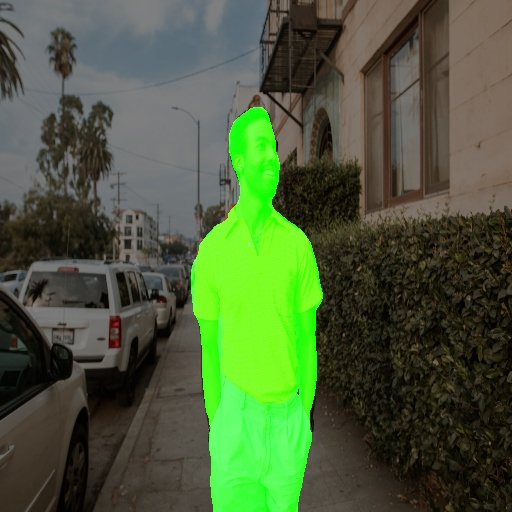
This is an easy scenario where we expect the model to perform well and it is doing so as well.

The next image contains multiple persons.

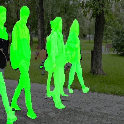
This time the scenario was a bit more challenging. Still, the model managed to perform quite well.

The final image is a difficult one with a crowded scene.

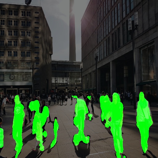
We can see that the model does not perform very well here. It fails when the scene is crowded and the persons are far away.

Inference on Videos using the Trained SegFormer-B1 Model

Now, let’s run inference on videos. This time, we will use the infer_video.py file. Instead of a directory containing images, we will provide the path to a video file.

python infer_video.py --input input/inference_data/videos/video_1.mp4 --imgsz 512 512

Here is the first result.

The results are good for this simple case. Both of the persons are being segmented by the model with very few artifacts. However, we can see that the model is also segmenting the dog as a person.

Let’s check out another case.

python infer_video.py --input input/inference_data/videos/video_2.mp4 --imgsz 512 512

Although the model is performing well in this case, the segmentation maps are not perfect when one person is very close to another.

Now, a final inference on a crowded scene.

python infer_video.py --input input/inference_data/videos/video_3.mp4 --imgsz 512 512

It is now evident that the model performs worse when the scene is crowded. It also suffers when the person is far away.

There are ways to mitigate such situations. We have trained on just 146 images. Transformer based models require more data to learn properly. If we can just increase the samples in the dataset, then also the model will start performing better without any other changes to the hyperparameters.

More Segmentation Blog Posts

Here are a few semantic segmentation blog posts that you will surely find interesting.

• Multi-Class Semantic Segmentation Training using PyTorch
• Person Segmentation with EfficientNet Lite Based Segmentation Models
• Semantic Segmentation for Flood Recognition using PyTorch
• Leaf Disease Segmentation using PyTorch DeepLabV3

Summary and Conclusion

We covered a lot in this blog post for training the SegFormer model on a person segmentation dataset. We started with the dataset discussion and then dived into the coding part. Starting with the dataset preparation, the model initialization, and finally the training process. After training, we also conducted inference experiments which revealed the strengths and weaknesses of the trained model. I hope that this blog post was worth your time.

If you have any doubts, thoughts, or suggestions, please leave them in the comment section. I will surely address them.

You can contact me using the Contact section. You can also find me on LinkedIn, and Twitter.

References

• mIoU script.