SegFormer for Semantic Segmentation

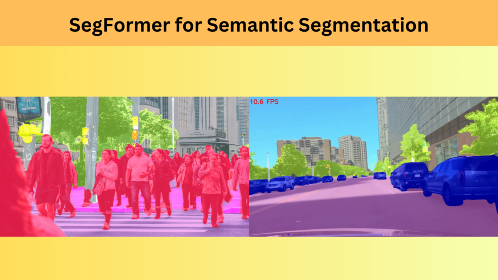
Semantic segmentation is one of the most important tasks in computer vision. It involves classifying each pixel in an image into a specific category. Until recently, CNNs have been in the lead in the task of semantic segmentation. However, like most tasks, transformer based architectures are slowly starting to take over. One such model is SegFormer. It is a transformer based semantic segmentation model with an All-MLP decoder. In this blog post, we will go through the summary of the SegFormer paper, and also carry out inference on images and videos using pretrained models.

SegFormer, as a semantic segmentation architecture, has proven to be highly useful. Starting from real-time inference to the best possible segmentation results, there are several pretrained models to choose from. We will take a look at all these components in this blog post.

What will we be covering in this article?

• We will start with the introduction of the SegFormer paper.
• We will follow this with the SegFormer architecture and its components.
• Next, the blog post will cover the advantages that SegFormer holds over other transformer based architecture.
• The model and paper discussion will end with a few points on the results that SegFormer delivers.
• Then, we will move on to the image and video inference using pretrained SegFormer models. We will use the Hugging Face Transformers library for this.

SegFormer

The SegFormer paper was introduced by Enze Xie et al. in 2021 under the title SegFormer: Simple and Efficient Design for Semantic Segmentation with Transformers.

The aim was to create a transformer based semantic segmentation model which was accurate as well as fast enough to run in real time. The paper has two main contributions:

• It has a novel Transformer encoder backbone that can output multiscale features.
• It has a simple MLP (Multi Layer Perceptron) decoder that aggregates features from different scales.

We will briefly discuss the above two points in the next section while covering the SegFormer architecture.

SegFormer Architecture

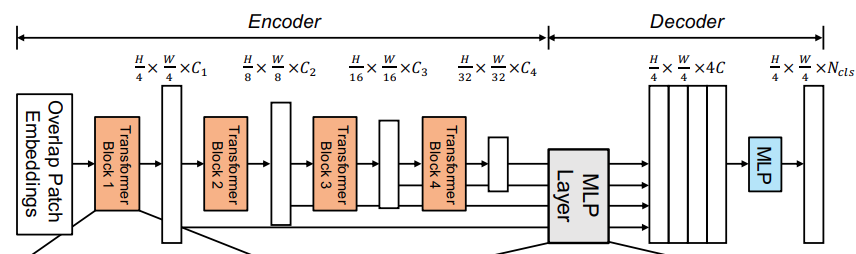
As we can see, like all semantic segmentation models, SegFormer also consists of an encoder and a decoder. The encoder is a Transformer encoder in this case and the decoder is an MLP decoder.

Further breaking down each transformer encoder block and the decoder block gives us a clearer picture.

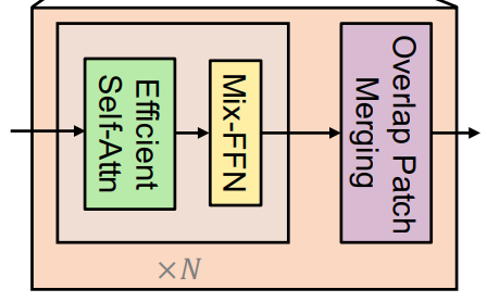
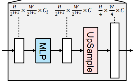
Each Transformer block contains Multi-head attention blocks, Feed Forward blocks, and Patch Merging blocks. Similarly, the decoder contains Linear layers and Upsampling layers.

The Transformer encoder breaks down each image into 4×4 patches. The Patch Merging layers help pool the features from different patches in an overlapping manner. This overlapping Patch Merging process helps preserve local features and continuity as well. This leads to better performance.

The backbone is called MiT (Mix Transformer Encoder). It is inspired by ViT while being more suitable for semantic segmentation. The authors propose backbones of different sizes, MiT-B0 to MiT-B5. These essentially have the same architecture but vary in scale.

Advantages of SegFormer Compared to Other Transformer Based Segmentation Models

Here are a few points where SegFormer shines compared to other Transformer based segmentation models.

• The backbone is pretrained only on ImageNet-1K while many others pretrain on the much larger ImageNet-22K. This shows a decrease in computational requirements.
• The hierarchical architecture of MiT can capture multiscale features. This leads to learning of both fine and coarse features of an image.
• SegFormer does not use Positional Encoding. Positional Encoding leads to worse test-time performance when the inference/test image resolution does not match the training image resolution.
• The computational overhead of the MLP decoder is negligible.

SegFormer Performance Comparison

In the final part of the paper summary, let’s take a look at how SegFormer performs compared to other models. The authors pretrain SegFormer on three datasets, Cityscapes, ADE-20K, and COCO-stuff.

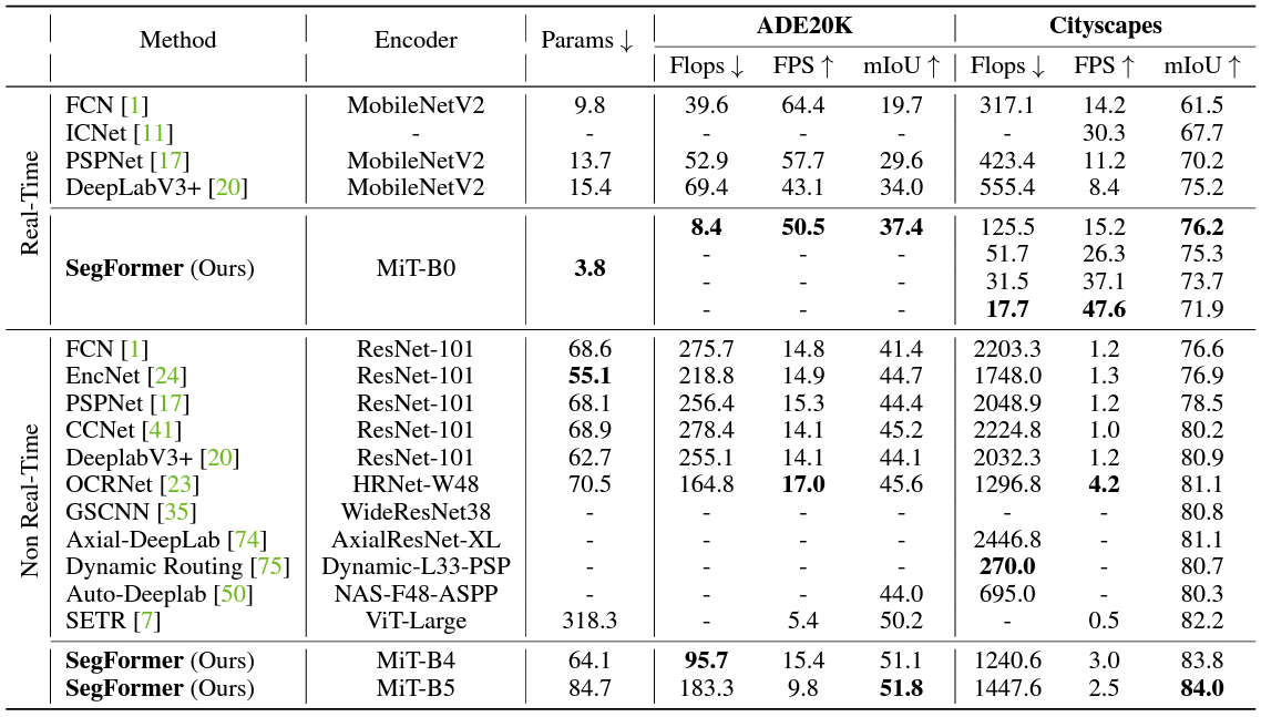
The above table compares different SegFormer models with other architectures on the ADE-20K and the Cityscapes dataset.

In the Real-Time section, we can see four rows. They are for four different resolutions where the short side of the image has been scaled to 1024, 768, 640, and 512 pixels respectively. We can see that even the slowest of SegFormer-B0 is faster than most of the other architectures while beating them at mIoU (Mean Intersection Over Union).

Furthermore, SegFormer-B4 and SegFormer-B5 while being the slowest of SegFormers, deliver the best accuracies compared to other semantic segmentation models.

We will conclude our discussion of the paper here. In the next section, we will see how to carry out inference on images and videos using SegFormer.

Want to know how to train DeepLabV3 for multi-class semantic segmentation? Take a look at Multi-Class Semantic Segmentation Training using PyTorch. In the post, we fine-tune the Torchvision DeepLabV3 model on the mini-KITTI dataset.

Inference using Segformer

Let’s move on to conduct inference experiments using the Transformer based semantic segmentation model.

Download Code

There are a few dependencies that we need to manage first.

We will use PyTorch for inference, so, first, we need to install it.

conda install pytorch torchvision torchaudio pytorch-cuda=11.7 -c pytorch -c nvidia

Next, we use the Hugging Face Transformer library to load the Segformer model. We need to install it as well.

pip install transformers

That’s it. There are other minor dependencies as well that you can install along the way if not already installed.

The Project Directory Structure

Before getting into the coding part, let’s check out the directory structure.

├── input
│   ├── images
│   └── videos
├── outputs
│   ├── segformer-b0_image_1.jpg
│   ...
│   └── segformer-b5_video_3.mp4
├── infer_image.py
├── infer_utils.py
├── infer_video.py
└── utils.py

• The input directory contains the images and videos that we will use for inference.
• All the outputs will be stored in the outputs directory.
• The parent project directory contains the Python files that we will need to carry out the inference.

Utilities

We need a few utilities and helper scripts along the way to carry out inference. The scripts that we will use here for inference support two pretrained models, Segformer-B0 and Segformer-B5, both pretrained on the Cityscapes dataset. B0 is the fastest model with lower quality segmentation outputs while B5 is the largest model with the best outputs. Along with that we also need the color palette for the segmentation masks for each class in the Cityscapes dataset. All of these are handled by the utils.py file.

model_mapper = {
    'segformer-b0': 'nvidia/segformer-b0-finetuned-cityscapes-768-768',
    'segformer-b5': 'nvidia/segformer-b5-finetuned-cityscapes-1024-1024'
}

cityscapes_classes = [
    "road",
    "sidewalk",
    "building",
    "wall",
    "fence",
    "pole",
    "traffic light",
    "traffic sign",
    "vegetation",
    "terrain",
    "sky",
    "person",
    "rider",
    "car",
    "truck",
    "bus",
    "train",
    "motorcycle",
    "bicycle",
]

cityscapes_palette = [
    [128, 64, 128],
    [244, 35, 232],
    [70, 70, 70],
    [102, 102, 156],
    [190, 153, 153],
    [153, 153, 153],
    [250, 170, 30],
    [220, 220, 0],
    [107, 142, 35],
    [152, 251, 152],
    [70, 130, 180],
    [220, 20, 60],
    [255, 0, 0],
    [0, 0, 142],
    [0, 0, 70],
    [0, 60, 100],
    [0, 80, 100],
    [0, 0, 230],
    [119, 11, 32],
]

The model_mapper dictionary creates a mapping between the model string name and the Hugging Face model name for downloading the model.

The cityscapes_palette is a list containing all the color values for each class. Although we don’t necessarily need the class names, still it is better to define them in the cityscapes_classes list.

Helper Scripts

We also need a few helper functions for inference. They are defined in the infer_utils.py file.

The first one is the predict() function to carry out inference.

import numpy as np
import cv2
import torch 
import torch.nn as nn

def predict(model, extractor, image, device):
    """
    :param model: The Segformer model.
    :param extractor: The Segformer feature extractor.
    :param image: The image in RGB format.
    :param device: The compute device.

    Returns:
        labels: The final labels (classes) in h x w format.
    """
    pixel_values = extractor(image, return_tensors='pt').pixel_values.to(device)
    with torch.no_grad():
        logits = model(pixel_values).logits

    # Rescale logits to original image size.
    logits = nn.functional.interpolate(
        logits,
        size=image.shape[:2],
        mode='bilinear',
        align_corners=False
    )

    # Get class labels.
    labels = torch.argmax(logits.squeeze(), dim=0)

    return labels

First, we import all the necessary packages.

The predict() function accepts the Segformer model, the Segformer feature extractor, the image, and the computation device as the parameters.

The very first step is to get the normalized pixel values using the extractor. These pixel values are passed down to the pretrained model and we obtain the logits from the model. However, these logits are downsampled ones. So, we upsample them to the original image size using the PyTorch interpolate method. Finally, we use argmax to obtain the class labels and return the label map.

The next two functions are helper functions to obtain the RGB segmentation map and the overlapped image and segmentation map.

def draw_segmentation_map(labels, palette):
    """
    :param labels: Label array from the model.Should be of shape 
        <height x width>. No channel information required.
    :param palette: List containing color information.
        e.g. [[0, 255, 0], [255, 255, 0]] 
    """
    # create Numpy arrays containing zeros
    # later to be used to fill them with respective red, green, and blue pixels
    red_map = np.zeros_like(labels).astype(np.uint8)
    green_map = np.zeros_like(labels).astype(np.uint8)
    blue_map = np.zeros_like(labels).astype(np.uint8)

    for label_num in range(0, len(palette)):
        index = labels == label_num
        red_map[index] = np.array(palette)[label_num, 0]
        green_map[index] = np.array(palette)[label_num, 1]
        blue_map[index] = np.array(palette)[label_num, 2]
        
    segmentation_map = np.stack([red_map, green_map, blue_map], axis=2)
    return segmentation_map

def image_overlay(image, segmented_image):
    """
    :param image: Image in RGB format.
    :param segmented_image: Segmentation map in RGB format. 
    """
    alpha = 0.5 # transparency for the original image
    beta = 1.0 # transparency for the segmentation map
    gamma = 0 # scalar added to each sum

    segmented_image = cv2.cvtColor(segmented_image, cv2.COLOR_RGB2BGR)
    image = np.array(image)
    image = cv2.cvtColor(image, cv2.COLOR_RGB2BGR)
    cv2.addWeighted(image, alpha, segmented_image, beta, gamma, image)
    return image

The draw_segmentation_map() accepts the class label map we obtained in the previous function and the color palette list as parameters. It converts the single channel label map into an RGB segmentation map and returns it.

The image_overlay() function accepts the original image and the segmentation map in RGB color format. It converts each of them into BGR format and creates an overlapping image.

Segformer Inference on Image

Let’s move forward with carrying out inference on images.

All the code for image inference will go into the infer_image.py file.

Starting with the import statements and defining the argument parser.

from transformers import (
    SegformerFeatureExtractor, 
    SegformerForSemanticSegmentation
)
from utils import model_mapper, cityscapes_palette
from infer_utils import (
    draw_segmentation_map, 
    image_overlay,
    predict
)

import argparse
import cv2
import glob
import os

parser = argparse.ArgumentParser()
parser.add_argument(
    '--input',
    help='path to the input image',
    default='input/images/image_1.jpg'
)
parser.add_argument(
    '--model',
    default='segformer-b0',
    help='the cityscapes pretrained segformer model name'
)
parser.add_argument(
    '--device',
    default='cuda:0',
    help='compute device, cpu or cuda'
)
args = parser.parse_args()

Here is a breakdown of the important modules that we import:

• SegformerFeatureExtractor and SegformerForSemanticSegmentation: We import these two from transformers to initialize the feature extractor and the Segformer model.
• model_mapper and cityscapes_palette: We need the model mapper dictionary to load the desired model according to the string passed in the command line. And the cityscapes_palette holds the RGB color values.
• draw_segmentation_map, image_overlay, and predict: These are functions that we defined above and will help us during inference.

We have the following command line arguments:

• --input: Path to the input image.
• --model: The model name. We can either pass segformer-b0 or segformer-b5.
• --device: The computation device. It is CUDA by default.

Moving forward, let’s define the output directory, the Segformer feature extractor, and the model.

out_dir = 'outputs'
os.makedirs(out_dir, exist_ok=True)

extractor = SegformerFeatureExtractor.from_pretrained(model_mapper[args.model])
model = SegformerForSemanticSegmentation.from_pretrained(model_mapper[args.model])
model.to(args.device).eval() 

Next, we read the image and carry on with the rest of the inference pipeline.

image = cv2.imread(args.input)
image = cv2.cvtColor(image, cv2.COLOR_BGR2RGB)

# Get labels.
labels = predict(model, extractor, image, args.device)

# Get segmentation map.
seg_map = draw_segmentation_map(
    labels.cpu(), cityscapes_palette
)
outputs = image_overlay(image, seg_map)
cv2.imshow('Image', outputs)
cv2.waitKey(0)

# Save path.
image_name = args.input.split(os.path.sep)[-1]
save_path = os.path.join(
    out_dir, args.model+'_'+image_name
)
cv2.imwrite(save_path, outputs)

Here are the steps that we follow for Segformer image inference.

• We convert the image to RGB format first.
• Then, we pass the image through the predict() function to get the single channel label map.
• Next, we pass the label map through the draw_segmentation_map() function to get the RGB segmentation map.
• This segmentation map and the original image are passed down to the image_overlay() function to get the final output.
• Finally, we save the image to the disk.

All the inference experiments were run on an RTX 3080 GPU with 10 GB VRAM.

Executing infer_image.py

Let’s execute the file and check some outputs.

We will start with Segformer-B0 and a simple image.

python infer_image.py --model segformer-b0 --input input/images/image_1.jpg

Here are the original and the overlayed images side-by-side.

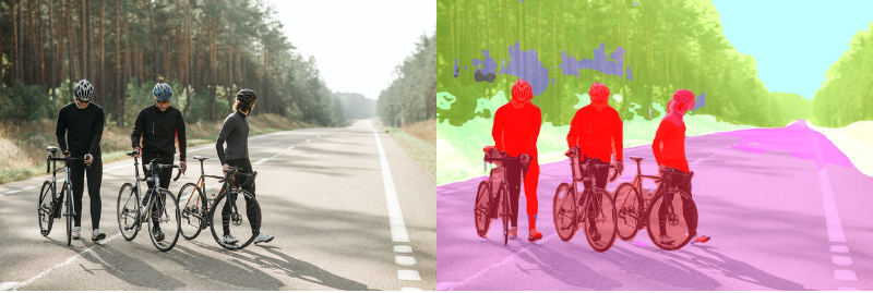
The model seems to be doing well. It is able to segment out the persons, bicycles, roads, and trees. There are a few artifacts though.

Let’s try another crowded scene with Segformer-B0.

python infer_image.py --model segformer-b0 --input input/images/image_3.jpg

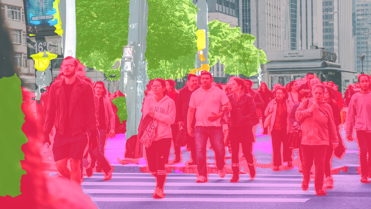
The Segformer-B0 model seems to be struggling when people are close to each other. Let’s check how Segformer-B5 performs.

python infer_image.py --model segformer-b5 --input input/images/image_3.jpg

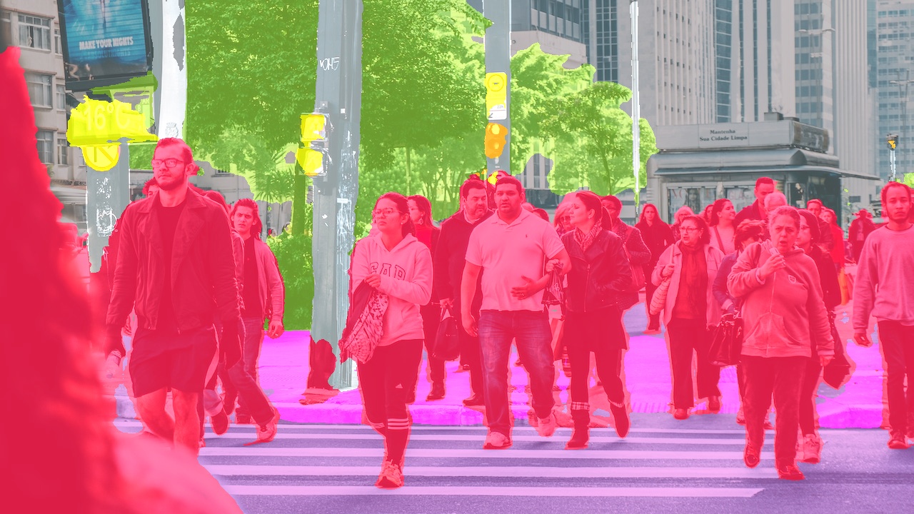
The results are excellent in this case. The larger model is able to segment out the persons, the road, and even the pavement clearly.

Segformer Video Inference

Moving ahead, we will write the code for video inference using Segformer.

The code for this will go into the infer_video.py file.

The initial parts where we import modules, define the argument parser, and initialize the model are going to be very similar to the image inference.

from transformers import (
    SegformerFeatureExtractor, 
    SegformerForSemanticSegmentation
)
from utils import model_mapper, cityscapes_palette
from infer_utils import (
    draw_segmentation_map, 
    image_overlay,
    predict
)

import argparse
import cv2
import time
import os

parser = argparse.ArgumentParser()
parser.add_argument(
    '--input',
    help='path to the input video',
    default='input/videos/video_1.mp4'
)
parser.add_argument(
    '--model',
    default='segformer-b0',
    help='the cityscapes pretrained segformer model name'
)
parser.add_argument(
    '--device',
    default='cuda:0',
    help='compute device, cpu or cuda'
)
args = parser.parse_args()

out_dir = 'outputs'
os.makedirs(out_dir, exist_ok=True)

extractor = SegformerFeatureExtractor.from_pretrained(model_mapper[args.model])
model = SegformerForSemanticSegmentation.from_pretrained(model_mapper[args.model])
model.to(args.device).eval()

Next, we read the video, capture the width & height of the frames, and define the output file name.

cap = cv2.VideoCapture(args.input)
frame_width = int(cap.get(3))
frame_height = int(cap.get(4))
vid_fps = int(cap.get(5))
save_name = args.input.split(os.path.sep)[-1].split('.')[0]
# Define codec and create VideoWriter object.
out = cv2.VideoWriter(f"{out_dir}/{args.model}_{save_name}.mp4", 
                    cv2.VideoWriter_fourcc(*'mp4v'), vid_fps, 
                    (frame_width, frame_height))

While carrying out inference, we will treat each frame of the video as an image. In that sense, after reading each frame, the rest of the inference pipeline will be similar to that of the image inference, although with some minor additions.

frame_count = 0
total_fps = 0
while cap.isOpened:
    ret, frame = cap.read()
    if ret:
        frame_count += 1
        image = frame
        image = cv2.cvtColor(image, cv2.COLOR_BGR2RGB)
    
        # Get labels.
        start_time = time.time()
        labels = predict(model, extractor, image, args.device)
        end_time = time.time()

        fps = 1 / (end_time - start_time)
        total_fps += fps
        
        # Get segmentation map.
        seg_map = draw_segmentation_map(
            labels.cpu(), cityscapes_palette
        )
        outputs = image_overlay(image, seg_map)
        cv2.putText(
            outputs,
            f"{fps:.1f} FPS",
            (15, 35),
            fontFace=cv2.FONT_HERSHEY_SIMPLEX,
            fontScale=1,
            color=(0, 0, 255),
            thickness=2,
            lineType=cv2.LINE_AA
        )
        out.write(outputs)
        cv2.imshow('Image', outputs)
        # Press `q` to exit
        if cv2.waitKey(1) & 0xFF == ord('q'):
            break
    else:
        break

# Release VideoCapture().
cap.release()
# Close all frames and video windows.
cv2.destroyAllWindows()

# Calculate and print the average FPS.
avg_fps = total_fps / frame_count
print(f"Average FPS: {avg_fps:.3f}")

After carrying out the inference, we also calculate the FPS and annotate it on the frame. This will help us compare the segmentation quality to speed between Segformer-B0 and Segformer-B5.

This brings us to the end of coding. We can now move on to executing the video inference script.

Executing infer_video.py

Starting with a video from the BDD10K dataset using the Segformer-B0 model.

python infer_video.py --model segformer-b0 --input input/videos/video_1.mov

The Segformer-B0 model is performing decently in this case. It is able to segment persons, the road, and cars. However, we can see some artifacts. One upside is that we are getting 55 FPS inference speed using the small model.

Let’s try the same video with Segformer-B5 now and check the performance.

python infer_video.py --model segformer-b5 --input input/videos/video_1.mov

Although the speed was reduced to just 10 FPS, the results are much better. The quality of the segmentation maps of the cars, road, and trees are higher. Not only that, the persons on the sidewalk are also segmented properly.

For the final inference experiment, we have a slightly challenging scenario of a highway scene. The vehicles are moving and appear to be somewhat at a distance. We will use the Segformer-B5 in this case.

python infer_video.py --model segformer-b5 --input input/videos/video_2.mp4

The limitations of the Segformer model are quite apparent here. Although the trees and roads appear to be properly segmented, we can see flickering in the segmentation maps of the moving vehicles.

Further Reading

We can also train semantic segmentation models for real-life use cases, like segmenting flooded areas or detecting diseased areas on leaves. In case you are interested, take a look at the following posts.

• Leaf Disease Segmentation using PyTorch DeepLabV3
• Semantic Segmentation for Flood Recognition using PyTorch

Summary and Conclusion

We dived into the Transformer based Segmentation model, Segformer in this blog post. Starting from the summary of the model architecture to inference, we covered a lot of topics. Along the way, we were able to figure out the strenghts and weaknesses of the model as well. In the next blog post, we will jump into fine-tuning the segformer model. I hope that this blog post was useful for you.

If you have any doubts, thoughts, or suggestions, please leave them in the comment section. I will surely address them.

You can contact me using the Contact section. You can also find me on LinkedIn, and Twitter.