Road Segmentation using SegFormer

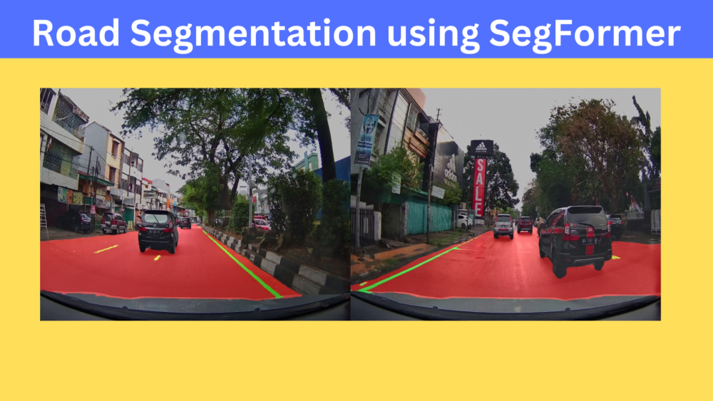
Semantic Segmentation has a lot of real-world applications. One such application is road and lane segmentation. This is also one of the important components in the deep learning models used for autonomous driving. However, choosing the right model for such tasks is equally important. A model that is performant yet fast enough to run in real time. To tackle a similar problem, in this blog post, we will carry out road segmentation using SegFormer.

We will use a SegFormer model and fine-tune it on a small road segmentation dataset. While doing so, we will also go through the dataset and model preparation. This will give us an overall idea of how to use SegFormer for real-world applications and which SegFormer model may suit the task.

Steps for road segmentation using SegFormer

• We will start with the dataset discussion. We will use a dataset containing a few hundred high-resolution images and segmentation maps for road and lane lines.
• Then we will discuss the configuration file. This will give us an idea of the color mapping for the segmentation maps.
• Next, we will move on to preparing the dataset where we need to define the augmentations for the semantic segmentation training process.
• After that, we need to prepare the SegFormer model. For the road segmentation task, we will specifically use the SegFormer-B3 model.
• The next step is training the model and analyzing the results.
• Finally, we will run inference on images and unseen videos.

The Road Segmentation Dataset

We will use the Semantic Segmentation Makassar(IDN) Road Dataset from Kaggle.

The dataset contains 374 high resolution images and segmentation maps. Each image is 2560×1600 pixels.

In its current state, the dataset does not contain a training and validation split. So, we will need to write a script to prepare the split.

It contains 4 classes including the background class.

• Background
• Roads
• Lane mark solid
• Lane mark dashed

You will get the following directory structure after downloading and extracting the dataset.

data_dataset_voc/
├── class_names.txt
├── colors.txt
├── JPEGImages
├── SegmentationClass
├── SegmentationClassPNG
└── SegmentationClassVisualization

The dataset gets extracted into the data_dataset_voc directory. The class_names.txt file contains the class names from the dataset. colors.txt file contains the color for each of the classes in the segmentation map. However, from the training process, I found that these colors are wrong and we will discuss the correct ones while preparing the configuration file.

Out of the directories, we are most interested in the JPEGImages and SegmentationClassPNG ones. They contain the RGB images and segmentation maps respectively.

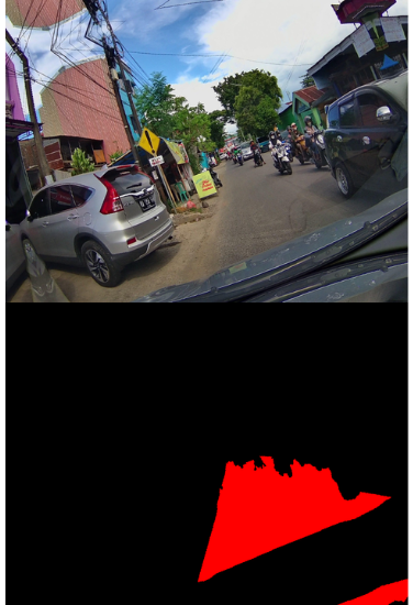
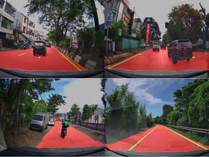
Here are some images and their respective segmentation maps.

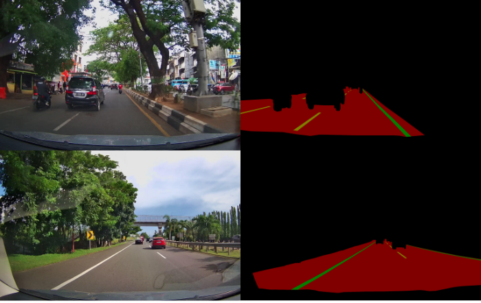
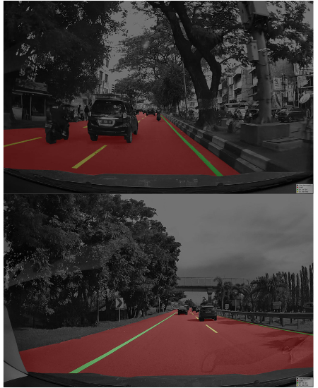
As we can see, the road is segmented in red color, solid lane lines in green, and dashed lane lines in yellow. To get a better idea, here are the images overlapped on the segmentation maps.

You may explore the dataset a bit more on your own before moving further.

Project Directory Structure

The following block shows the entire project’s directory structure.

├── input
│   ├── data_dataset_voc
│   │   ├── JPEGImages
│   │   ├── SegmentationClass
│   │   ├── SegmentationClassPNG
│   │   ├── SegmentationClassVisualization
│   │   ├── class_names.txt
│   │   └── colors.txt
│   ├── inference_data
│   │   └── videos
│   ├── train
│   │   ├── images
│   │   └── masks
│   └── valid
│       ├── images
│       └── masks
├── outputs
│   ├── final_model
│   ├── inference_results_video
│   ├── model_iou
│   ├── model_loss
│   ├── valid_preds [75 entries exceeds filelimit, not opening dir]
│   ├── accuracy.png
│   ├── loss.png
│   └── miou.png
├── config.py
├── datasets.py
├── engine.py
├── infer_image.py
├── infer_video.py
├── metrics.py
├── model.py
├── split_data.py
├── train.py
└── utils.py

• The input directory contains the original dataset as well as the dataset after creating the split. The train and valid directories contain the respective images and segmentation maps.
• In the outputs directory, we have the results from the training and inference experiments. These include the trained models, plots, and video inference results.
• In the parent project directory, we have several Python files. We will discuss the important components of the files as we discuss the coding section.

The trained model weights and inference files are provided via the download section. You can use them directly to run inference.

Libraries and Dependencies

There are quite a few major dependencies for training SegFormer for road segmentation.

First, we need PyTorch which we can install using the conda command.

conda install pytorch==2.0.1 torchvision==0.15.2 torchaudio==2.0.2 pytorch-cuda=11.7 -c pytorch -c nvidia

Second, we need two libraries from Hugging Face.

pip install transformers
pip install accelerate -U 

And finally, we need Albumentations for image augmentations.

pip install -U albumentations --no-binary qudida,albumentations

Road Segmentation using SegFormer-B3

Let’s start the discussion of the coding section for training SegFomer-B3 on the road segmentation dataset.

The code that we need to train the SegFormer-B3 remains largely the same as we discussed in the post where we trained the SegFormer model for person segmentation. So, we will just discuss the most important parts here. If you need to get an in-depth explanation, please go through the training SegFormer post. Everything is discussed in detail in the post.

Download Code

Creating the Training and Validation Split for the Road Segmentation Dataset

As we discussed earlier, in the current state our dataset does not contain a training and a validation split. The code in the split_data.py file contains the code to create the splits.

To create the splits, we can execute the following command.

python split_data.py

This will create the train and valid subdirectories inside the input directory. As of this, we have 299 training samples and 74 validation samples to train the SegFormer-B3 model for road segmentation.

The Configuration File

Next is the configuration file. It contains the class names, the color mapping for creating the dataset and data loaders, and the color mapping for visualization. The configuration code is present in the config.py file.

ALL_CLASSES = [
    '_background_',
    'road',
    'lm_solid',
    'lm_dashed'
]

LABEL_COLORS_LIST = [
    [0,0,0],
    [128,0,0],
    [0,128,0],
    [128,128,0]
]

VIS_LABEL_MAP = [
    [0,0,0],
    [128,0,0],
    [0,128,0],
    [128,128,0]
]

The LABEL_COLOR_LIST will be used in the datasets.py to create the segmentation labels according to the segmentation map colors. If we want, we can also visualize the predicted segmentation maps with different colors during the inference stage. These colors are defined in the VIS_LABEL_MAP. As of now, we keep both the color palette the same.

The Dataset Preparation and Augmentation

While preparing the dataset for road segmentation, one of the most important parts is the augmentations. All the dataset preparation code is present in the datasets.py file.

The following code block shows the augmentations and transformations that we apply to the training and validation datasets.

def train_transforms(img_size):
    """
    Transforms/augmentations for training images and masks.

    :param img_size: Integer, for image resize.
    """
    train_image_transform = A.Compose([
        A.Resize(img_size[1], img_size[0], always_apply=True),
        A.HorizontalFlip(p=0.5),
        A.RandomBrightnessContrast(p=0.2),
        A.Rotate(limit=25),
    ], is_check_shapes=False)
    return train_image_transform

def valid_transforms(img_size):
    """
    Transforms/augmentations for validation images and masks.

    :param img_size: Integer, for image resize.
    """
    valid_image_transform = A.Compose([
        A.Resize(img_size[1], img_size[0], always_apply=True),
    ], is_check_shapes=False)
    return valid_image_transform

For the training set, we apply the following augmentations using Albumentations:

• Horizontal flipping with a probability of 0.5.
• Randomizing the brightness and contrast with a probability of 0.2.
• Rotating the samples with a degree range of -25 to +25.

It is important to note that geometric augmentations like flipping and rotation will be applied to both, images and masks. Whereas color level augmentations like changing the brightness and contrast will only be applied to the images. Thanks to Albumentations, this process is seamless.

Let’s take a look at the augmented images and masks.

The above figure shows a few images and their respective segmentation maps after augmentation. Such augmentations will prevent overfitting and allow the model to learn various new features that are not part of the original dataset.

The Utility Scripts and Helper Functions

The utils.py file contains several helper functions and classes. The following are some of the important ones among them.

def set_class_values(all_classes, classes_to_train):
    """
    This (`class_values`) assigns a specific class label to the each of the classes.
    For example, `animal=0`, `archway=1`, and so on.

    :param all_classes: List containing all class names.
    :param classes_to_train: List containing class names to train.
    """
    class_values = [all_classes.index(cls.lower()) for cls in classes_to_train]
    return class_values

def get_label_mask(mask, class_values, label_colors_list):
    """
    This function encodes the pixels belonging to the same class
    in the image into the same label

    :param mask: NumPy array, segmentation mask.
    :param class_values: List containing class values, e.g car=0, bus=1.
    :param label_colors_list: List containing RGB color value for each class.
    """
    label_mask = np.zeros((mask.shape[0], mask.shape[1]), dtype=np.uint8)
    for value in class_values:
        for ii, label in enumerate(label_colors_list):
            if value == label_colors_list.index(label):
                label = np.array(label)
                label_mask[np.where(np.all(mask == label, axis=-1))[:2]] = value
    label_mask = label_mask.astype(int)
    return label_mask

We need to convert the RGB segmentation map to 2D segmentation maps or label maps to train the semantic segmentation model. The set_class_values and get_label_mask functions help with that. The former assigns an integer value to each class and the latter replaces the RBG mask values in the segmentation map with the class value for a particular class.

class SaveBestModel:
    """
    Class to save the best model while training. If the current epoch's 
    validation loss is less than the previous least less, then save the
    model state.
    """
    def __init__(self, best_valid_loss=float('inf')):
        self.best_valid_loss = best_valid_loss
        
    def __call__(
        self, current_valid_loss, epoch, model, out_dir, name='model'
    ):
        if current_valid_loss < self.best_valid_loss:
            self.best_valid_loss = current_valid_loss
            print(f"\nBest validation loss: {self.best_valid_loss}")
            print(f"\nSaving best model for epoch: {epoch+1}\n")
            model.save_pretrained(os.path.join(out_dir, name))

class SaveBestModelIOU:
    """
    Class to save the best model while training. If the current epoch's 
    IoU is higher than the previous highest, then save the
    model state.
    """
    def __init__(self, best_iou=float(0)):
        self.best_iou = best_iou
        
    def __call__(self, current_iou, epoch, model, out_dir, name='model'):
        if current_iou > self.best_iou:
            self.best_iou = current_iou
            print(f"\nBest validation IoU: {self.best_iou}")
            print(f"\nSaving best model for epoch: {epoch+1}\n")
            model.save_pretrained(os.path.join(out_dir, name))

def save_model(model, out_dir, name='model'):
    """
    Function to save the trained model to disk.
    """
    model.save_pretrained(os.path.join(out_dir, name))

We have three utilities for saving the model.

The SaveBestModel will save the model whenever the current validation loss is less than the previous least loss.

The SaveBestModelIOU class will save the model whenever the model reaches a new validation mean IoU value.

Finally, the save_model function will save the model once the training is completed.

The Engine File For Training and Validation

The engine.py file contains the training and validation functions.

Although we will not discuss the entirety of the training and validation functions here, there are a few things to note.

outputs = model(pixel_values=pixel_values, labels=target)
##### BATCH-WISE LOSS #####
loss = outputs.loss

The above code snippet shows the forward pass through one batch of the data. This remains the same for both, the training and validation loops.

The outputs that we get from the model contain both, the loss values as well as the logits. We can directly use this loss value for backward propagation and weight update. Alternatively, we also have the option to write our custom function and calculate the loss based on the logits.

Metrics for Monitoring the Training

We rely on the Mean IoU metric to obtain the best model. The metrics.py file contains the code to calculate the mean IoU and pixel accuracy.

The values returned are used by the train and validate functions in the engine.py file.

Training the SegFormer-B3 Model

We can execute the train.py file to start the training process. Although it supports numerous command line arguments, we will only discuss those that we use here.

All training and inference experiments were carried out on a machine with 10 GB RTX 3080 GPU, 10th generation i7 CPU, and 32 GB of RAM.

python train.py --lr 0.0001 --batch 2 --imgsz 800 600 --epochs 75

We are using a base learning or 0.0001, batch size of 2, image resolution of 800×600, and will be training for 75 epochs.

Here is the log from the final epoch.

EPOCH: 75
Training
100%|████████████████████| 150/150 [00:47<00:00,  3.18it/s]                                                                                                                                                        
Validating
100%|████████████████████| 37/37 [00:04<00:00,  8.80it/s]                                                                                                                                                          

Best validation IoU: 0.7499804704256651

Saving best model for epoch: 75

Train Epoch Loss: 0.0546, Train Epoch PixAcc: 0.9706, Train Epoch mIOU: 0.747937
Valid Epoch Loss: 0.0166, Valid Epoch PixAcc: 0.9686 Valid Epoch mIOU: 0.749980
--------------------------------------------------
TRAINING COMPLETE

We obtained the mode with the best IoU of 75% on the last epoch.

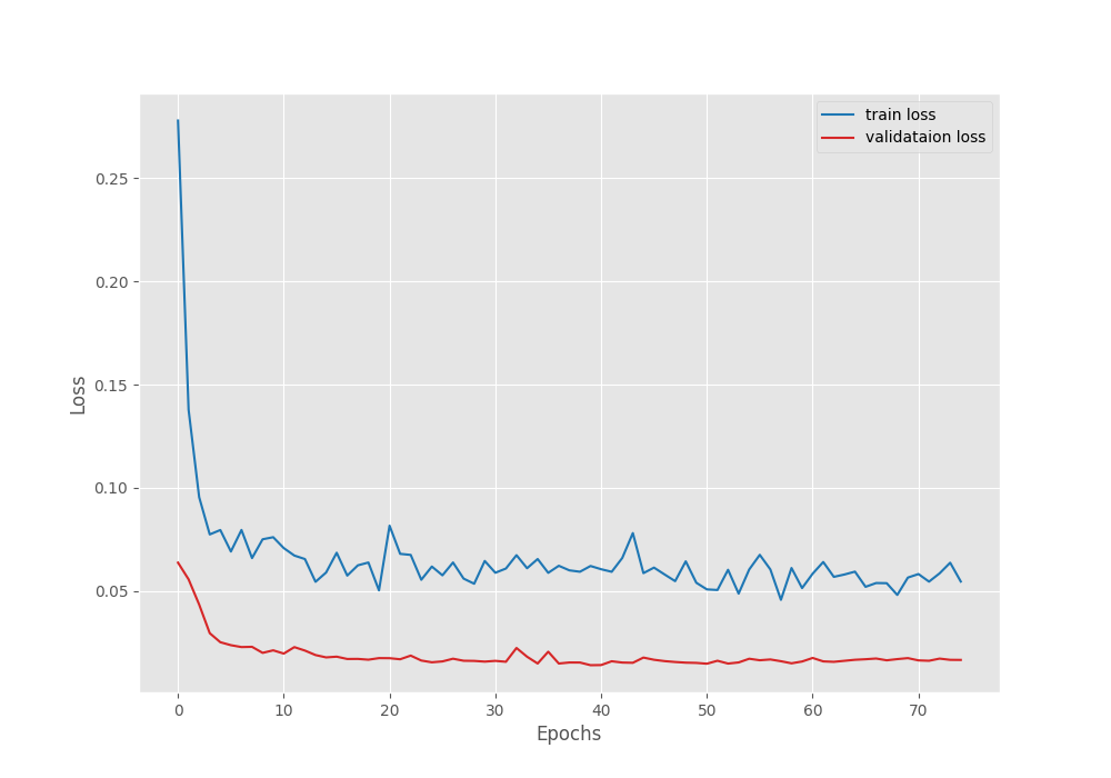
The validation loss seems to be increasing a bit in the final few epochs. Mostly, applying a learning rate scheduler will mitigate that.

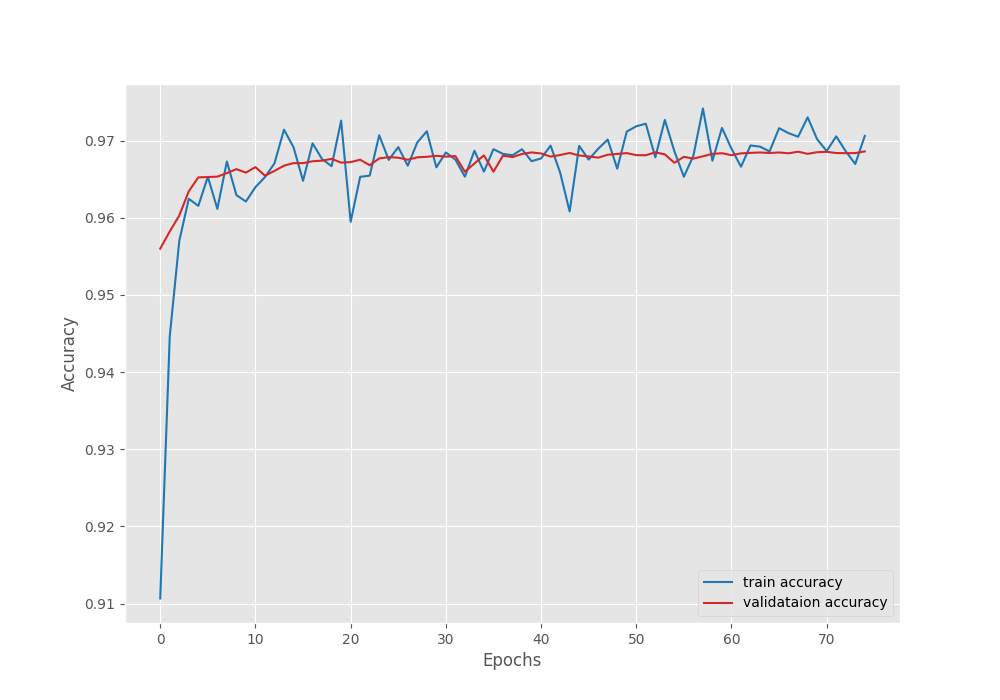
The validation pixel accuracy seems to be increasing till the end of the training.

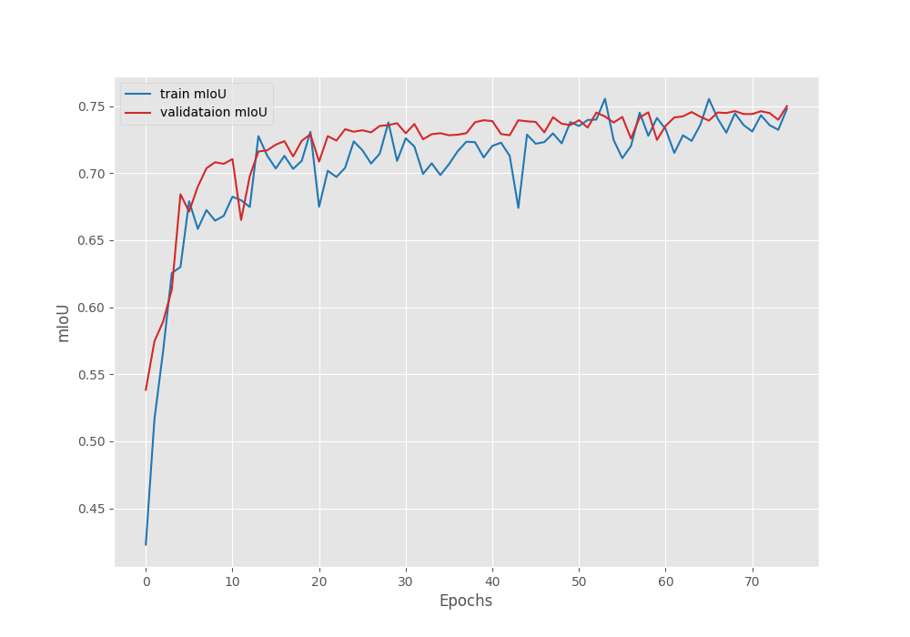
The mean IoU plot is also improving till the training is finished.

From the metrics and loss plots it is evident that if we reduce the base learning (say, by a factor of 10), then most probably, we can train for a bit longer.

Road Segmentation Inference using the Trained SegFormer-B3 Model

We can now use the model saved with the best IoU for inference in images and videos. The code for both is present in the infer_image.py and infer_video.py scripts.

Although we will not go into the details of the code, there is one important point to take note of here. As we have trained and saved our model using the Transformers library, the loading of the model will be slightly different. We need to use the following syntax to load the model.

model = SegformerForSemanticSegmentation.from_pretrained('outputs/model_iou')

We need to use the SegformerForSemanticSegmentation class from the transformers library and have to give the path to the directory where the model is saved. The model will be loaded according to the configuration file inside the directory.

Let’s now move forward with the image inference. For image inference, we will use the validation images. To carry out image inference, we can execute the following command.

python infer_image.py --input input/train/images/ --imgsz 800 600

We are providing the path to the input directory containing the images and the image size is 800×600 which matches the training image size.

The model is segmenting the road and lane lines really well.

However, we will get more insights once we run inference on some unseen videos. Let’s run video inference now.

python infer_video.py --input input/inference_data/videos/video_3.mov --imgsz 800 600

For video inference, we need to provide the path to a video. Here are the results.

Although not perfect, the results are more than decent here. The model is able to segment the road and the lane lines. The model is getting confused between the solid lane lines and dashed lane lines in some cases. But we can fix it by training it with more data. Furthermore, it is running at an average of 32 FPS on an RTX 3080 GPU.

Summary and Conclusion

We trained a SegFormer-B3 model for road segmentation in this blog post. We started with the discussion and preparation of the dataset and moved to the model initialization. After training, we also ran inference on images and videos. That gave us a better idea of the model’s performance on unseen data. I hope that this article was worth your time.

If you have any doubts, thoughts, or suggestions, please leave them in the comment section. I will try my best to answer them.

You can contact me using the Contact section. You can also find me on LinkedIn, and Twitter.