Fine-Tuning FCOS using PyTorch

FCOS is a fully convolutional anchor-free single-stage object detection model. It was first introduced in Fully Convolutional One-Stage Object Detection with a follow-up for the anchor free mechanism in A Simple and Strong Anchor-free Object Detector. The authors of both papers were Zhi Tian, Chunhua Shen, Hao Chen, and Tong He. In this blog post, we will fine-tune the FCOS model from Torchvision. We will create an end-to-end pipeline for fine-tuning FCOS using PyTorch.

We will cover the following points in this blog post.

• We will start with a discussion of the object detection dataset that we will use to fine-tune the FCOS model.
• Then we will move on to the coding part. Here we will discuss all the important code details. These include:
  • The configuration file.
  • The dataset preparation.
  • Preparing the FCOS model.
  • The custom utilities that we will need along the way.
  • And the training script.
• After training the FCOS model, we will analyze the results.
• Finally, we will run inference on images and videos using the trained model.

The Smoke Detection Dataset

In this blog post, we will use a smoke detection dataset for fine-tuning the FCOS model. The original dataset is available on Kaggle. However, the dataset that we will use here is available through the downloadable zip file and already has a training and validation split.

The dataset annotation file is present in XML format and the class name is smoke. There are 665 training samples and 72 validation samples. Here is the data directory structure.

smoke_pascal_voc/
├── train
│   ├── annotations
│   └── images
└── valid
    ├── annotations
    └── images

The training and validation samples are present in their respective directories. Each of these contains subdirectories for images and annotations.

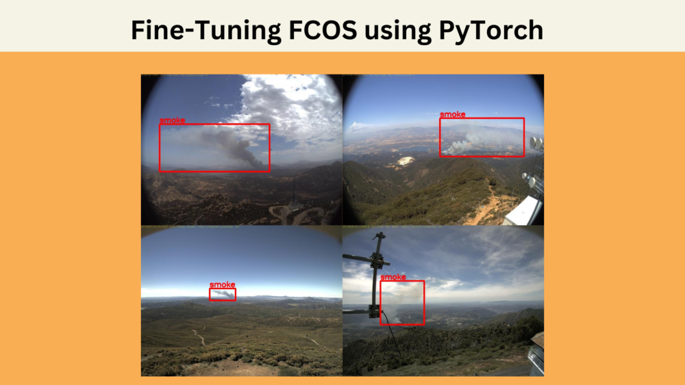
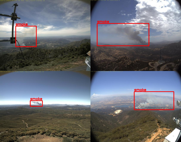
Here are a few samples from the dataset along with their annotations.

As we can see, the smoke images have been captured from a camera. Further, most of the scenes appear to be in a hilly area. So, it may become a bit challenging for our model to learn diverse features.

The Project Directory Structure

The following block shows the entire project directory structure.

├── inference_outputs
│   ├── images
│   │   ├── ck0k99e6p79go0944lmxivkmv_jpeg.jpg
│   │   ...
│   │   └── ck0kfnjva6jp60838d6vqyxq2_jpeg.jpg
│   └── videos
│       ├── video_1.mp4
│       └── video_2.mp4
├── input
│   ├── inference_data
│   │   └── videos
│   └── smoke_pascal_voc
│       ├── train
│       └── valid
├── outputs
│   ├── best_model.pth
│   ├── last_model.pth
│   ├── map.png
│   └── train_loss.png
├── config.py
├── custom_utils.py
├── datasets.py
├── inference_image.py
├── inference_video.py
├── model.py
└── train.py

• The input directory contains the training and inference data. We have already seen the structure of the training directory in the previous section.
• The outputs directory contains the plots and trained models from the training experiment.
• In the inference_outputs directory, we have the inference results for both images and videos.
• In the parent project directory, we have all the Python files that we need for training the FCOS model and running inference experiments.

The dataset, Python files, and the trained model will be available via the download section of this blog post. You can either run inference directly using the trained weights or run the training experiments yourself as well.

Frameworks and Dependencies

The codebase for this blog post has been developed using PyTorch 2.0.1. We also use Albumentations for image augmentations, and Torchmetrics for the evaluation of the mAP metric. Do ensure that you have these installed in case you run the training experiment.

If you want to use the COCO pretrained FCOS model in PyTorch for inference, then surely check out Anchor Free Object Detection Inference using FCOS. It will help you get started with FCOS.

Fine-Tuning FCOS for Smoke Detection using PyTorch

We will go through all the important components of the code for training FCOS. Let’s begin with the configuration file.

Download Code

Configuration File for Training FCOS

All the training related configurations are present in the config.py file. Let’s check out the content of the file first.

import torch

BATCH_SIZE = 16 # Increase / decrease according to GPU memeory.
RESIZE_TO = 640 # Resize the image for training and transforms.
NUM_EPOCHS = 40 # Number of epochs to train for.
NUM_WORKERS = 4 # Number of parallel workers for data loading.

DEVICE = torch.device('cuda') if torch.cuda.is_available() else torch.device('cpu')

# Training images and XML files directory.
TRAIN_IMG = 'input/smoke_pascal_voc/train/images'
TRAIN_ANNOT = 'input/smoke_pascal_voc/train/annotations'
# Validation images and XML files directory.
VALID_IMG = 'input/smoke_pascal_voc/valid/images'
VALID_ANNOT = 'input/smoke_pascal_voc/valid/annotations'

# Classes: 0 index is reserved for background.
CLASSES = [
    '__background__', 
    'smoke'
]

NUM_CLASSES = len(CLASSES)

# Whether to visualize images after crearing the data loaders.
VISUALIZE_TRANSFORMED_IMAGES = False

# Location to save model and plots.
OUT_DIR = 'outputs'

First, we define the batch size, image resizing resolution, number of epochs to train for, and the number of workers for parallel processing. You can modify the batch size according to the GPU memory that you have available. We also define the computation device which is CUDA by default.

Second, we define the paths to the training and validation images as well as the annotation files.

Then we define the class names and the number of classes. Do note that the CLASSES also include a mandatory __background__ class along with the object class. This brings the total number of classes to 2.

Next, we have a VISUALIZE_TRANSFORMED_IMAGES variable. If this is True, then a few data loader samples will be visualized on the screen before the training starts.

Finally, we have the output directory path where all the training related outputs will be saved.

Preparing the FCOS Model

Now, let’s prepare the FCOS model. The code for this goes into the model.py file.

import torchvision
import torch

from functools import partial
from torchvision.models.detection.fcos import FCOSClassificationHead

def create_model(num_classes=91, min_size=640, max_size=640):
    model = torchvision.models.detection.fcos_resnet50_fpn(
        weights='DEFAULT'
    )
    num_anchors = model.head.classification_head.num_anchors

    model.head.classification_head = FCOSClassificationHead(
        in_channels=256,
        num_anchors=num_anchors,
        num_classes=num_classes,
        norm_layer=partial(torch.nn.GroupNorm, 32)
    )

    model.transform.min_size = (min_size, )
    model.transform.max_size = max_size
    for param in model.parameters():
        param.requires_grad = True
    return model

The function create_model creates an instance of the FCOS model, using a ResNet50 backbone, combined with a Feature Pyramid Network (FPN) to enhance the feature representations at different scales. The function has options for the number of classes (num_classes), and minimum and maximum sizes (min_size and max_size) for the images being processed.

Inside the function, an initial FCOS model is instantiated with torchvision.models.detection.fcos_resnet50_fpn(weights='DEFAULT'). This leverages the pretrained weights provided by torchvision if available.

Then, we replace the classification head of the model with a new FCOSClassificationHead. This customization allows one to specify the number of output classes and adjust other internal parameters. Notably, the norm_layer is set to use Group Normalization with 32 groups using the partial function from the functools module.

Lastly, we set the image transformation sizes according to the passed parameters. This ensures that the input images are resized correctly during training. The loop at the end ensures that all model parameters are trainable.

The final model contains around 32 million parameters.

Defining Custom Utilities

Any object detection training requires a lot of custom utilities, classes, and helper functions. For our use case, we have the utilities code in custom_utils.py.

import albumentations as A
import cv2
import numpy as np
import torch
import matplotlib.pyplot as plt

from albumentations.pytorch import ToTensorV2
from config import DEVICE, CLASSES

plt.style.use('ggplot')

# This class keeps track of the training and validation loss values
# and helps to get the average for each epoch as well.
class Averager:
    def __init__(self):
        self.current_total = 0.0
        self.iterations = 0.0
        
    def send(self, value):
        self.current_total += value
        self.iterations += 1
    
    @property
    def value(self):
        if self.iterations == 0:
            return 0
        else:
            return 1.0 * self.current_total / self.iterations
    
    def reset(self):
        self.current_total = 0.0
        self.iterations = 0.0

class SaveBestModel:
    """
    Class to save the best model while training. If the current epoch's 
    validation mAP @0.5:0.95 IoU higher than the previous highest, then save the
    model state.
    """
    def __init__(
        self, best_valid_map=float(0)
    ):
        self.best_valid_map = best_valid_map
        
    def __call__(
        self, 
        model, 
        current_valid_map, 
        epoch, 
        OUT_DIR,
    ):
        if current_valid_map > self.best_valid_map:
            self.best_valid_map = current_valid_map
            print(f"\nBEST VALIDATION mAP: {self.best_valid_map}")
            print(f"\nSAVING BEST MODEL FOR EPOCH: {epoch+1}\n")
            torch.save({
                'epoch': epoch+1,
                'model_state_dict': model.state_dict(),
                }, f"{OUT_DIR}/best_model.pth")

The Averager class is a simple utility to track the average of a series of values. This class is particularly useful for monitoring the average training loss across epochs. It allows for easy addition of new values and computes the current average on demand. The SaveBestModel class is designed to persist the model with the best validation performance. As training progresses, it checks if the latest model has a higher mean Average Precision (mAP) than the previous best and saves it if true.

def collate_fn(batch):
    """
    To handle the data loading as different images may have different number 
    of objects and to handle varying size tensors as well.
    """
    return tuple(zip(*batch))

# Define the training tranforms.
def get_train_transform():
    return A.Compose([
        A.HorizontalFlip(p=0.5),
        A.Blur(blur_limit=3, p=0.1),
        A.MotionBlur(blur_limit=3, p=0.1),
        A.MedianBlur(blur_limit=3, p=0.1),
        A.RandomBrightnessContrast(p=0.3),
        A.RandomGamma(p=0.3),
        ToTensorV2(p=1.0),
    ], bbox_params={
        'format': 'pascal_voc',
        'label_fields': ['labels']
    })

# Define the validation transforms.
def get_valid_transform():
    return A.Compose([
        ToTensorV2(p=1.0),
    ], bbox_params={
        'format': 'pascal_voc', 
        'label_fields': ['labels']
    })


def show_tranformed_image(train_loader):
    """
    This function shows the transformed images from the `train_loader`.
    Helps to check whether the tranformed images along with the corresponding
    labels are correct or not.
    Only runs if `VISUALIZE_TRANSFORMED_IMAGES = True` in config.py.
    """
    if len(train_loader) > 0:
        for i in range(1):
            images, targets = next(iter(train_loader))
            images = list(image.to(DEVICE) for image in images)
            targets = [{k: v.to(DEVICE) for k, v in t.items()} for t in targets]
            boxes = targets[i]['boxes'].cpu().numpy().astype(np.int32)
            labels = targets[i]['labels'].cpu().numpy().astype(np.int32)
            sample = images[i].permute(1, 2, 0).cpu().numpy()
            sample = cv2.cvtColor(sample, cv2.COLOR_RGB2BGR)
            for box_num, box in enumerate(boxes):
                cv2.rectangle(sample,
                            (box[0], box[1]),
                            (box[2], box[3]),
                            (0, 0, 255), 2)
                cv2.putText(sample, CLASSES[labels[box_num]], 
                            (box[0], box[1]-10), cv2.FONT_HERSHEY_SIMPLEX, 
                            1.0, (0, 0, 255), 2)
            cv2.imshow('Transformed image', sample)
            cv2.waitKey(0)
            cv2.destroyAllWindows()

Several data transformation functions are present to preprocess the input data for both training and validation.

The get_train_transform and get_valid_transform functions leverage the albumentations library to define bounding box augmentation strategies for training and straightforward transformations for validation, respectively. These augmentations include operations like horizontal flipping, blurring, and adjusting brightness and contrast. Additionally, the collate_fn function ensures consistent data batching, given that different images might contain varying numbers of annotated objects.

The utility also includes a visualization function, show_tranformed_image, that displays augmented training images with their associated bounding boxes, helping to ensure that the transformations and annotations are applied correctly.

def save_model(epoch, model, optimizer):
    """
    Function to save the trained model till current epoch, or whenver called
    """
    torch.save({
                'epoch': epoch+1,
                'model_state_dict': model.state_dict(),
                'optimizer_state_dict': optimizer.state_dict(),
                }, 'outputs/last_model.pth')

def save_loss_plot(
    OUT_DIR, 
    train_loss_list, 
    x_label='iterations',
    y_label='train loss',
    save_name='train_loss'
):
    """
    Function to save both train loss graph.
    
    :param OUT_DIR: Path to save the graphs.
    :param train_loss_list: List containing the training loss values.
    """
    figure_1 = plt.figure(figsize=(10, 7), num=1, clear=True)
    train_ax = figure_1.add_subplot()
    train_ax.plot(train_loss_list, color='tab:blue')
    train_ax.set_xlabel(x_label)
    train_ax.set_ylabel(y_label)
    figure_1.savefig(f"{OUT_DIR}/{save_name}.png")
    print('SAVING PLOTS COMPLETE...')

def save_mAP(OUT_DIR, map_05, map):
    """
    Saves the [email protected] and [email protected]:0.95 per epoch.
    :param OUT_DIR: Path to save the graphs.
    :param map_05: List containing mAP values at 0.5 IoU.
    :param map: List containing mAP values at 0.5:0.95 IoU.
    """
    figure = plt.figure(figsize=(10, 7), num=1, clear=True)
    ax = figure.add_subplot()
    ax.plot(
        map_05, color='tab:orange', linestyle='-', 
        label='[email protected]'
    )
    ax.plot(
        map, color='tab:red', linestyle='-', 
        label='[email protected]:0.95'
    )
    ax.set_xlabel('Epochs')
    ax.set_ylabel('mAP')
    ax.legend()
    figure.savefig(f"{OUT_DIR}/map.png")

Lastly, the script contains utilities for saving model progress and visualization. The save_model function saves the model and optimizer states for a given epoch, while the save_loss_plot and save_mAP functions save the training loss and mAP values, respectively.

Dataset Preparation for Fine-Tuning FCOS

Object detection requires extensive data preparation code. This holds true when fine-tuning FCOS as well. All the dataset preparation code is present in the datasets.py file.

Let’s start with the imports and the custom dataset class.

import torch
import cv2
import numpy as np
import os
import glob as glob

from xml.etree import ElementTree as et
from torch.utils.data import Dataset, DataLoader
from custom_utils import collate_fn, get_train_transform, get_valid_transform

# The dataset class.
class CustomDataset(Dataset):
    def __init__(
        self, 
        img_path, 
        annot_path, 
        width, 
        height, 
        classes, 
        transforms=None
    ):
        self.transforms = transforms
        self.img_path = img_path
        self.annot_path = annot_path
        self.height = height
        self.width = width
        self.classes = classes
        self.image_file_types = ['*.jpg', '*.jpeg', '*.png', '*.ppm', '*.JPG']
        self.all_image_paths = []
        
        # Get all the image paths in sorted order.
        for file_type in self.image_file_types:
            self.all_image_paths.extend(glob.glob(os.path.join(self.img_path, file_type)))
        self.all_images = [image_path.split(os.path.sep)[-1] for image_path in self.all_image_paths]
        self.all_images = sorted(self.all_images)

    def __getitem__(self, idx):
        # Capture the image name and the full image path.
        image_name = self.all_images[idx]
        image_path = os.path.join(self.img_path, image_name)

        # Read and preprocess the image.
        image = cv2.imread(image_path)
        image = cv2.cvtColor(image, cv2.COLOR_BGR2RGB).astype(np.float32)
        image_resized = cv2.resize(image, (self.width, self.height))
        image_resized /= 255.0
        
        # Capture the corresponding XML file for getting the annotations.
        annot_filename = os.path.splitext(image_name)[0] + '.xml'
        annot_file_path = os.path.join(self.annot_path, annot_filename)
        
        boxes = []
        labels = []
        tree = et.parse(annot_file_path)
        root = tree.getroot()
        
        # Original image width and height.
        image_width = image.shape[1]
        image_height = image.shape[0]
        
        # Box coordinates for xml files are extracted 
        # and corrected for image size given.
        for member in root.findall('object'):
            # Get label and map the `classes`.
            labels.append(self.classes.index(member.find('name').text))
            
            # Left corner x-coordinates.
            xmin = int(member.find('bndbox').find('xmin').text)
            # Right corner x-coordinates.
            xmax = int(member.find('bndbox').find('xmax').text)
            # Left corner y-coordinates.
            ymin = int(member.find('bndbox').find('ymin').text)
            # Right corner y-coordinates.
            ymax = int(member.find('bndbox').find('ymax').text)
            
            # Resize the bounding boxes according 
            # to resized image `width`, `height`.
            xmin_final = (xmin/image_width)*self.width
            xmax_final = (xmax/image_width)*self.width
            ymin_final = (ymin/image_height)*self.height
            ymax_final = (ymax/image_height)*self.height

            # Check that max coordinates are at least one pixel
            # larger than min coordinates.
            if xmax_final == xmin_final:
                xmin_final -= 1
            if ymax_final == ymin_final:
                ymin_final -= 1
            # Check that all coordinates are within the image.
            if xmax_final > self.width:
                xmax_final = self.width
            if ymax_final > self.height:
                ymax_final = self.height
            
            boxes.append([xmin_final, ymin_final, xmax_final, ymax_final])
        
        # Bounding box to tensor.
        boxes = torch.as_tensor(boxes, dtype=torch.float32)
        # Area of the bounding boxes.
        area = (boxes[:, 3] - boxes[:, 1]) * (boxes[:, 2] - boxes[:, 0]) if len(boxes) > 0 \
            else torch.as_tensor(boxes, dtype=torch.float32)
        # No crowd instances.
        iscrowd = torch.zeros((boxes.shape[0],), dtype=torch.int64)
        # Labels to tensor.
        labels = torch.as_tensor(labels, dtype=torch.int64)

        # Prepare the final `target` dictionary.
        target = {}
        target["boxes"] = boxes
        target["labels"] = labels
        target["area"] = area
        target["iscrowd"] = iscrowd
        image_id = torch.tensor([idx])
        target["image_id"] = image_id

        # Apply the image transforms.
        if self.transforms:
            sample = self.transforms(image = image_resized,
                                     bboxes = target['boxes'],
                                     labels = labels)
            image_resized = sample['image']
            target['boxes'] = torch.Tensor(sample['bboxes'])
        
        if np.isnan((target['boxes']).numpy()).any() or target['boxes'].shape == torch.Size([0]):
            target['boxes'] = torch.zeros((0, 4), dtype=torch.int64)
        return image_resized, target

    def __len__(self):
        return len(self.all_images)

The main component of the code is the CustomDataset class which inherits from PyTorch’s Dataset class. Within its constructor, the class takes in paths to the images and their corresponding XML annotations, desired image dimensions, class names, and optional transformations.

The class reads and stores paths to image files and, for any given index, it reads the corresponding image, resizes it, and extracts its bounding box annotations from the XML files. We adjust the bounding boxes for the resized image dimensions and transform them into PyTorch tensors. The dataset can then return the processed image and its annotations as a dictionary of tensors.

We apply the augmentations to the training set only.

# Prepare the final datasets and data loaders.
def create_train_dataset(img_dir, annot_dir, classes, resize=640):
    train_dataset = CustomDataset(
        img_dir, 
        annot_dir, 
        resize, 
        resize, 
        classes, 
        get_train_transform()
    )
    return train_dataset
def create_valid_dataset(img_dir, annot_dir, classes, resize=640):
    valid_dataset = CustomDataset(
        img_dir, 
        annot_dir, 
        resize, 
        resize, 
        classes, 
        get_valid_transform()
    )
    return valid_dataset
def create_train_loader(train_dataset, batch_size, num_workers=0):
    train_loader = DataLoader(
        train_dataset,
        batch_size=batch_size,
        shuffle=True,
        num_workers=num_workers,
        collate_fn=collate_fn,
        drop_last=False
    )
    return train_loader
def create_valid_loader(valid_dataset, batch_size, num_workers=0):
    valid_loader = DataLoader(
        valid_dataset,
        batch_size=batch_size,
        shuffle=False,
        num_workers=num_workers,
        collate_fn=collate_fn,
        drop_last=False
    )
    return valid_loader

To facilitate the training and validation processes, we have the following utility functions: create_train_dataset, create_valid_dataset, create_train_loader, and create_valid_loader.

These functions wrap around the CustomDataset class and the PyTorch DataLoader to offer an easy way to instantiate datasets and data loaders for training and validation.

They account for different configurations like image resizing, applying different transformations, and setting batch sizes.

# execute `datasets.py`` using Python command from 
# Terminal to visualize sample images
# USAGE: python datasets.py
if __name__ == '__main__':
    # sanity check of the Dataset pipeline with sample visualization
    from config import TRAIN_IMG, TRAIN_ANNOT, RESIZE_TO, CLASSES
    from custom_utils import show_tranformed_image
    dataset = create_train_dataset(
        TRAIN_IMG, TRAIN_ANNOT, CLASSES, RESIZE_TO
    )
    loader = create_train_loader(dataset, batch_size=2, num_workers=0)
    show_tranformed_image(loader)

Finally, we have some utilities within the main code block. If we execute the datasets.py directly, then we can visualize a few transformed images from the data loader. This is helpful for debugging and ensuring that all the transformations and augmentations are indeed correct.

This brings us to the end of the dataset preparation. Let’s move on to the training script now.

The Training Script for Fine-Tuning FCOS

The training script is quite extensive and connects all the components that we have defined till now. All of the code for the training script is present in the train.py file.

Starting with the import statements.

from config import (
    DEVICE, 
    NUM_CLASSES,
    CLASSES,
    BATCH_SIZE,
    NUM_EPOCHS, 
    OUT_DIR,
    VISUALIZE_TRANSFORMED_IMAGES, 
    NUM_WORKERS,
    RESIZE_TO,
    TRAIN_IMG,
    TRAIN_ANNOT,
    VALID_IMG,
    VALID_ANNOT
)
from model import create_model
from custom_utils import (
    Averager, 
    SaveBestModel, 
    save_model, 
    save_loss_plot,
    save_mAP
)
from tqdm.auto import tqdm
from datasets import (
    create_train_dataset, 
    create_valid_dataset, 
    create_train_loader, 
    create_valid_loader
)
from torchmetrics.detection.mean_ap import MeanAveragePrecision
from torch.optim.lr_scheduler import MultiStepLR

import torch
import matplotlib.pyplot as plt
import time
import os

plt.style.use('ggplot')

seed = 42
torch.manual_seed(seed)
torch.cuda.manual_seed(seed)
torch.cuda.manual_seed_all(seed) 

We import all the necessary modules including the configurations. These configurations will be necessary while preparing the datasets and data loaders.

Note that we also import the MeanAveragePrecision class from torchmetrics. We will monitor the validation mAP metric to evaluate and save the best model.

We also set the seed to make the training runs reproducible.

Next, we have the training and validation functions.

# Function for running training iterations.
def train(train_data_loader, model):
    print('Training')
    model.train()
    
     # initialize tqdm progress bar
    prog_bar = tqdm(train_data_loader, total=len(train_data_loader))
    
    for i, data in enumerate(prog_bar):
        optimizer.zero_grad()
        images, targets = data
        
        images = list(image.to(DEVICE) for image in images)
        targets = [{k: v.to(DEVICE) for k, v in t.items()} for t in targets]
        loss_dict = model(images, targets)

        losses = sum(loss for loss in loss_dict.values())
        loss_value = losses.item()

        train_loss_hist.send(loss_value)

        losses.backward()
        optimizer.step()
    
        # update the loss value beside the progress bar for each iteration
        prog_bar.set_description(desc=f"Loss: {loss_value:.4f}")
    return loss_value

# Function for running validation iterations.
def validate(valid_data_loader, model):
    print('Validating')
    model.eval()
    
    # Initialize tqdm progress bar.
    prog_bar = tqdm(valid_data_loader, total=len(valid_data_loader))
    target = []
    preds = []
    for i, data in enumerate(prog_bar):
        images, targets = data
        
        images = list(image.to(DEVICE) for image in images)
        targets = [{k: v.to(DEVICE) for k, v in t.items()} for t in targets]
        
        with torch.no_grad():
            outputs = model(images, targets)

        # For mAP calculation using Torchmetrics.
        #####################################
        for i in range(len(images)):
            true_dict = dict()
            preds_dict = dict()
            true_dict['boxes'] = targets[i]['boxes'].detach().cpu()
            true_dict['labels'] = targets[i]['labels'].detach().cpu()
            preds_dict['boxes'] = outputs[i]['boxes'].detach().cpu()
            preds_dict['scores'] = outputs[i]['scores'].detach().cpu()
            preds_dict['labels'] = outputs[i]['labels'].detach().cpu()
            preds.append(preds_dict)
            target.append(true_dict)
        #####################################

    metric.reset()
    metric.update(preds, target)
    metric_summary = metric.compute()
    return metric_summary

While training, we enable the model.train(). This ensures that the model directly returns the training loss when forward passing the images and labels through the model.

In the training function, we also keep track of the average loss value per epoch and return it at the end.

In the validate function, we keep the model in eval() mode. Because of this, the model returns the detection predictions. We use these prediction values to calculate the mAP metric on each epoch. We return the mAP value so that we can compare the value for the best mAP.

if __name__ == '__main__':
    os.makedirs('outputs', exist_ok=True)
    train_dataset = create_train_dataset(TRAIN_IMG, TRAIN_ANNOT, CLASSES, RESIZE_TO)
    valid_dataset = create_valid_dataset(VALID_IMG, VALID_ANNOT, CLASSES, RESIZE_TO)
    train_loader = create_train_loader(train_dataset, BATCH_SIZE, NUM_WORKERS)
    valid_loader = create_valid_loader(valid_dataset, BATCH_SIZE, NUM_WORKERS)
    print(f"Number of training samples: {len(train_dataset)}")
    print(f"Number of validation samples: {len(valid_dataset)}\n")

    # Initialize the model and move to the computation device.
    model = create_model(
        num_classes=NUM_CLASSES, min_size=RESIZE_TO, max_size=RESIZE_TO
    )
    model = model.to(DEVICE)
    print(model)
    # Total parameters and trainable parameters.
    total_params = sum(p.numel() for p in model.parameters())
    print(f"{total_params:,} total parameters.")
    total_trainable_params = sum(
        p.numel() for p in model.parameters() if p.requires_grad)
    print(f"{total_trainable_params:,} training parameters.")
    params = [p for p in model.parameters() if p.requires_grad]
    optimizer = torch.optim.SGD(
        params, lr=0.002, momentum=0.9, weight_decay=0.0005
    )
    scheduler = MultiStepLR(
        optimizer=optimizer, milestones=[20], gamma=0.1, verbose=True
    )

    # To monitor training loss
    train_loss_hist = Averager()
    # To store training loss and mAP values.
    train_loss_list = []
    map_50_list = []
    map_list = []

    metric = MeanAveragePrecision()

    # Mame to save the trained model with.
    MODEL_NAME = 'model'

    # Whether to show transformed images from data loader or not.
    if VISUALIZE_TRANSFORMED_IMAGES:
        from custom_utils import show_tranformed_image
        show_tranformed_image(train_loader)

    # To save best model.
    save_best_model = SaveBestModel()

    # Training loop.
    for epoch in range(NUM_EPOCHS):
        print(f"\nEPOCH {epoch+1} of {NUM_EPOCHS}")

        # Reset the training loss histories for the current epoch.
        train_loss_hist.reset()

        # Start timer and carry out training and validation.
        start = time.time()
        train_loss = train(train_loader, model)
        metric_summary = validate(valid_loader, model)
        print(f"Epoch #{epoch+1} train loss: {train_loss_hist.value:.3f}")   
        print(f"Epoch #{epoch+1} [email protected]:0.95: {metric_summary['map']}")
        print(f"Epoch #{epoch+1} [email protected]: {metric_summary['map_50']}")   
        end = time.time()
        print(f"Took {((end - start) / 60):.3f} minutes for epoch {epoch}")

        train_loss_list.append(train_loss)
        map_50_list.append(metric_summary['map_50'])
        map_list.append(metric_summary['map'])

        # save the best model till now.
        save_best_model(
            model, float(metric_summary['map']), epoch, 'outputs'
        )
        # Save the current epoch model.
        save_model(epoch, model, optimizer)

        # Save loss plot.
        save_loss_plot(OUT_DIR, train_loss_list)

        # Save mAP plot.
        save_mAP(OUT_DIR, map_50_list, map_list)
        scheduler.step()

Finally, we have the main code block. Here, we first create the datasets and data loaders according to the configurations.

Then, we initialize the model, the optimizer, and the multi-step learning rate scheduler. We use the SGD optimizer with an initial learning rate of 0.002 and reduce it by a factor of 10 after 20 epochs.

Next, we initialize the Averager class and a few lists to store the loss and mAP values. Along with that, we also initialize the MeanAveragePrecision class for calculating the mAP.

We start the training loop and after each loop, we print the mAP metric and try to save the best model according to the mAP value.

Running the Training Experiment

The training experiments were carried out on a machine with 10 GB RTX 3080 GPU, i7 10th generation CPU, and 32 GB of RAM.

To start the training, we need to execute the following command from the parent project directory.

python train.py 

EPOCH 1 of 40
Training
Loss: 1.7578: 100%|████████████████████████████████████████████████████████████████████████████████████████████████████████████████████████████████████████████████████████████████| 42/42 [00:24<00:00,  1.69it/s]
Validating
100%|████████████████████████████████████████████████████████████████████████████████████████████████████████████████████████████████████████████████████████████████████████████████| 5/5 [00:01<00:00,  2.69it/s]
Epoch #1 train loss: 2.602
Epoch #1 [email protected]:0.95: 0.028769461438059807
Epoch #1 [email protected]: 0.10572247952222824
Took 0.449 minutes for epoch 0

BEST VALIDATION mAP: 0.028769461438059807

SAVING BEST MODEL FOR EPOCH: 1

SAVING PLOTS COMPLETE...
Adjusting learning rate of group 0 to 2.0000e-03.
.
.
.
EPOCH 37 of 40
Training
Loss: 0.7736: 100%|████████████████████████████████████████████████████████████████████████████████████████████████████████████████████████████████████████████████████████████████| 42/42 [00:23<00:00,  1.76it/s]
Validating
100%|████████████████████████████████████████████████████████████████████████████████████████████████████████████████████████████████████████████████████████████████████████████████| 5/5 [00:02<00:00,  2.10it/s]
Epoch #37 train loss: 0.818
Epoch #37 [email protected]:0.95: 0.5782641172409058
Epoch #37 [email protected]: 0.9663254618644714
Took 0.440 minutes for epoch 36

BEST VALIDATION mAP: 0.5782641172409058

SAVING BEST MODEL FOR EPOCH: 37

SAVING PLOTS COMPLETE...
Adjusting learning rate of group 0 to 2.0000e-04.

The best model was saved after 37 epochs. Here, we have an mAP of 57% which is quite good.

Let’s take a look at the mAP and loss graphs.

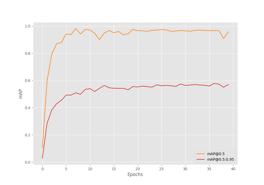
From the graph, we can see that the mAP plot fluctuates less after 20 epochs. This is where we apply the learning rate scheduler.

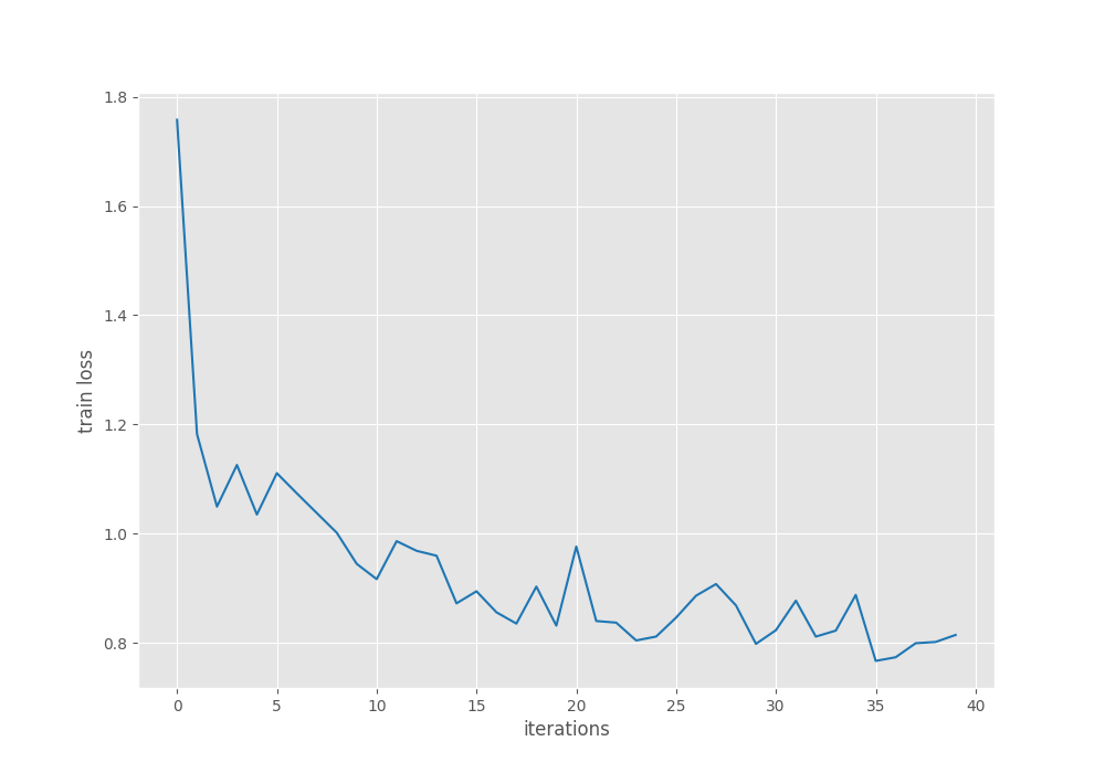
The training loss plot seems a bit unstable till the end of training. Nonetheless, we have our best model with us now that we can use for inference.

Inference using the Fine-Tuned FCOS Model

We will run inference on images and videos. We will not go through the code in detail for the inference scripts. They are straightforward PyTorch detection inference scripts. However, you can take a look at the inference_image.py and inference_video.py files before moving forward.

Starting with the image inference. In this case, we will use the validation images as inference data. The inference_image.py script accepts the following command line arguments.

• --input: The path to the directory containing images.
• --imgsz: An integer value for resizing the image. A value of 640 will resize the images into 640×640 dimensions.
• --threshold: The confidence threshold for visualization.

Let’s execute the script now.

python inference_image.py --input input/smoke_pascal_voc/valid/images/ --threshold 0.5 --imgsz 640

We are providing the path to the inference data directory, with a threshold of 0.5, and resizing the images to 640×640 resolution.

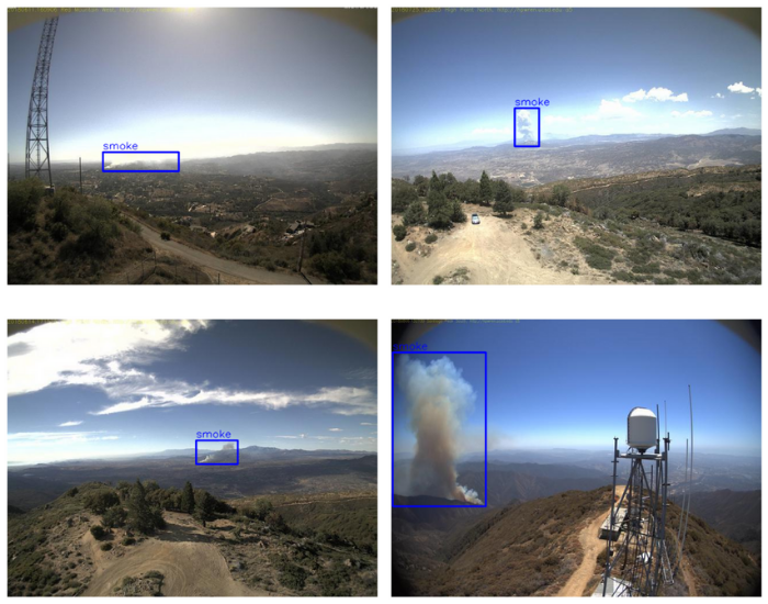
Here are some good inference results.

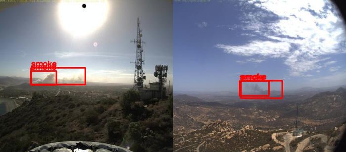
The model does not detect the smoke in all the images perfectly. The following are some images with false detections.

Moving forward, let’s run inference on videos. The inference_video.py script also accepts the same arguments. However, the --input argument accepts the path to a video file.

Starting with the first video.

python inference_video.py --input input/inference_data/videos/video_1.mp4 --threshold 0.6 --imgsz 640

We are getting an FPS of 52 on the RTX 3080 GPU. Regarding the detections, we can see that the model does not detect the right part of the smoke until some time. Also, there are a few false detections.

Let’s run inference on the second video. This time with a confidence score of 0.6 to mitigate false detections.

python inference_video.py --input input/inference_data/videos/video_2.mp4 --threshold 0.5 --imgsz 640

Although initially, the model was detecting the smoke, it does not any more when the helicopter enters the scene.

Takeaways

Fine-tuning FCOS provided us with some valuable lessons. It was one of the first few anchor free object detection methods. It is not as robust as the recent methods such as DETR or YOLOv8. We got to see firsthand, although the model was performing well on validation data, the performance on out of distribution videos was not good.

This raises the need to keep ourselves updated with the newer detection techniques that are coming out so that we can leverage the best in object detection.

Summary and Conclusion

In this blog post, we fine-tuned the FCOS model. We started with the dataset discussion, the configuration file, preparing the model, running the training experiments, and inferencing. The results provided us with first-hand experience about the limitations of the FCOS model. I hope that this article was worth your time.

If you have any doubts, thoughts, or suggestions, please leave them in the comment section. I will surely address them.

You can contact me using the Contact section. You can also find me on LinkedIn, and Twitter.

References

• FCOS: Fully Convolutional One-Stage Object Detection
• FCOS: A simple and strong anchor-free object detector
• Smoke Pascal VOC dataset