Fine-Tuning SegFormer for Multi-Class Segmentation

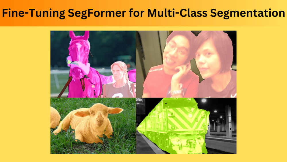
We will continue with the SegFormer series with this blog post. In this blog post, we will be fine-tuning SegFormer on a multi-class segmentation dataset.

In the previous two blog posts, we covered inference using SegFormer and training SegFormer on a binary segmentation dataset.

Here, we will take a step forward and will be fine-tuning one of the SegFormer models on a much more challenging multi-class semantic segmentation dataset.

We will cover the following in this blog post.

• We will start with a discussion of the dataset. While doing so, getting to know the classes and visualizing the images & segmentation maps is a vital part. The dataset that we are going to use is the Pascal VOC semantic segmentation dataset.
• Next, we will move on to the coding section. As most of the code is similar to the previous post, we will cover only the important parts here.
• Then we will train the model and analyze the results.
• After training, we will run inference on images and videos.

The Pascal VOC Semantic Segmentation Dataset

The Pascal VOC semantic segmentation dataset contains a subset of images from the detection set. But instead of bounding box annotations, it contains semantic segmentation annotations.

The dataset version that we are going to use here is present here on Kaggle. It contains 1464 training samples and 1449 validation samples. The classes are the same as in the detection set with the exception of an extra background class. Here are the classes.

• background
• aeroplane
• bicycle
• bird
• boat
• bottle
• bus
• car
• cat
• chair
• cow
• dining table
• dog
• horse
• motorbike
• person
• potted plant
• sheep
• sofa
• train
• tv/monitor

There are a total of 21 classes including the background class.

Downloading and extracting the dataset reveals the following directory structure.

voc_2012_segmentation_data/
├── train_images
├── train_labels
├── valid_images
└── valid_labels

The dataset gets extracted into the voc_2012_segmentation_data directory. The train_images and train_labels contain the training images and the segmentation maps in PNG format. Similarly, valid_images and valid_labels contain the validation samples.

Following are some images and the ground truth segmentation map from the dataset.

As we can see, the images contain several objects in varying scenes. While this is good for the model to learn features from different types of scenarios, only 1464 training samples may hinder the learning of the segmentation map of each class properly.

The Project Directory Structure

Here is the entire project directory structure.

├── input
│   ├── inference_data
│   └── voc_2012_segmentation_data
│       ├── train_images
│       ├── train_labels
│       ├── valid_images
│       └── valid_labels
├── outputs
│   ├── final_model
│   ├── inference_results_image [36 entries exceeds filelimit, not opening dir]
│   ├── inference_results_video
│   ├── model_iou
│   ├── model_loss
│   ├── valid_preds [50 entries exceeds filelimit, not opening dir]
│   ├── accuracy.png
│   ├── loss.png
│   └── miou.png
├── config.py
├── datasets.py
├── engine.py
├── infer_image.py
├── infer_video.py
├── metrics.py
├── model.py
├── train.py
└── utils.py

• The input directory contains the Pascal VOC segmentation dataset that we saw in the previous section. Along with that, it also contains the data for inference.
• The outputs directory contains all the saved models, intermediate results from the training, and the inference results as well.
• Directly inside the parent project directory, we have the Python files. We will go through the important ones in the coding section.

The trained model (best IoU) and inference data will be available for download via the download section. You can run inference directly using these. To train the model yourself, you will need to download the dataset and arrange it in the above structure.

Installing Dependencies

We need the following libraries and frameworks for training and inference. All the training commands are expected to be run within an Anaconda environment.

• PyTorch

conda install pytorch==2.0.1 torchvision==0.15.2 torchaudio==2.0.2 pytorch-cuda=11.7 -c pytorch -c nvidia

• Hugging Face Transformers and Accelerate. We need the Transformers library to access the SegFormer model.

pip install transformers
pip install accelerate -U 

• Albumentations for data augmentation.

pip install -U albumentations --no-binary qudida,albumentations

With this, we complete the setup of the project. Let’s now move towards the technical discussion.

Fine-Tuning SegFormer on Pascal VOC Dataset

Most of the code that we need for fine-tuning the SegFormer model will be similar to the previous post where we covered training SegFormer on a person segmentation dataset. Each of the files needed for training is discussed in detail in that post. For that reason, here, we will discuss only the most important coding parts and some of the changes that were needed for multi-class segmentation training.

Download Code

The Configuration File

The configuration file is one of the most important ones among all of the Python files. This contains the class information, the pixel color for each class during training, and also during visualization. All of this information goes into the config.py file.

ALL_CLASSES = [
    'background',
    'aeroplane',
    'bicycle',
    'bird',
    'boat',
    'bottle',
    'bus',
    'car',
    'cat',
    'chair',
    'cow',
    'dining table',
    'dog',
    'horse',
    'motorbike',
    'person',
    'potted plant',
    'sheep',
    'sofa',
    'train',
    'tv/monitor'
]

LABEL_COLORS_LIST = [
    [0, 0, 0],
    [128, 0, 0],
    [0, 128, 0],
    [128, 128, 0],
    [0, 0, 128],
    [128, 0, 128],
    [0, 128, 128], 
    [128, 128, 128],
    [64, 0, 0],
    [192, 0, 0],
    [64, 128, 0],
    [192, 128, 0],
    [64, 0, 128],
    [192, 0, 128],
    [64, 128, 128],
    [192, 128, 128],
    [0, 64, 0],
    [128, 64, 0],
    [0, 192, 0],   
    [128, 192, 0],
    [0, 64, 128]
]

VIS_LABEL_MAP = [
    [0, 0, 0],
    [128, 0, 0],
    [0, 128, 0],
    [128, 128, 0],
    [0, 0, 128],
    [128, 0, 128],
    [0, 128, 128], 
    [128, 128, 128],
    [64, 0, 0],
    [192, 0, 0],
    [64, 128, 0],
    [192, 128, 0],
    [64, 0, 128],
    [192, 0, 128],
    [64, 128, 128],
    [192, 128, 128],
    [0, 64, 0],
    [128, 64, 0],
    [0, 192, 0],   
    [128, 192, 0],
    [0, 64, 128]
]

The LABEL_COLORS_LIST contains the RGB color mapping for each class. During visualization inference, we can change the color if we want in the VIS_LABEL_MAP. But for simplicity, we keep it the same.

Helper Functions and Classes

We need a lot of helper functions, utilities, and custom classes to train the model. These include:

• The set_class_values function which assigns an integer to each class.
• The get_label_mask which encodes an individual class within an image with the same pixel values.
• draw_translucent_seg_maps function to save one predicted sample from the validation loop while training.
• Custom classes and functions to save the best model according to the highest IoU, and least loss, and also to save the final model.
• Further, we also have functions that help during inference to create the RGB segmentation map from the predicted output and overlay the segmentation map on top of the image.

You may go through the utils.py file to get a detailed look at the code.

The Dataset Preparation Code

All the dataset preparation code resides in the datasets.py file. As with any deep learning problem, it is one of the most important files.

For the training set, we apply the following augmentation using Albumentations.

• Horizontal flipping with a probability of 0.5.
• Randomizing the brightness and contrast with a probability of 0.2.
• Rotating the samples by 25 degrees.

Note that horizontal flipping and rotation are geometric transformations. So, they will be applied to both images and masks. While the randomization of the contrast is a pixel-level augmentation that is only applied to the images.

For both, the training and validation datasets, we resize the samples into a fixed size. As usual, we do not apply any augmentation to the validation samples.

For the data loaders, we use 8 parallel workers. You can increase or decrease the value depending on the number of logical processors that you have.

The Evaluation Metrics

The IoUEval class in the metrics.py file computes both, the pixel accuracy, and the mean IoU (mIoU). However, we are choosing the mIoU as our primary metric. While saving the model, we will save one of the models according to the highest mIoU.

The Training and Validation Functions

We have very detailed training and validation functions in the engine.py file.

The train function gets the normalized image and segmentation maps from each batch of the data and forward passes it through the model. The model outputs the loss and the logits from the last layer.

For each batch, we do backpropagation and update the model weights. We also upsample the logits of each batch to the same size as the data loader masks. We use this to calculate the mean IoU and the pixel accuracy.

In the end, we return the epoch-wise loss, pixel accuracy, and the mIoU.

The validate function is almost the same but we do not need any backpropagation or updation of the model weights. Further, we call the draw_translucent_seg_maps to save one sample from the validation set on each epoch with the predicted segmentation map overlapped on the image. This will give us a real-time idea of the model performance on each epoch.

The SegForer Model

We will use the SegFormer-B5 model for fine-tuning on the Pascal VOC segmentation dataset. The model.py contains the model preparation model.

from transformers import SegformerForSemanticSegmentation

def segformer_model(classes):
    model = SegformerForSemanticSegmentation.from_pretrained(
        'nvidia/mit-b5',
        num_labels=len(classes),
    )
    return model

We use the SegformerForSemanticSegmentation from the transformers library to load the model. This model has not been fine-tuned on any dataset. Instead, it only contains an ImageNet1K pretrained backbone and we will fine-tune it on the Pascal VOC dataset. The backbone is the MiT-B5 (Mix Transformer). The final model contains 84.6 million parameters.

If you wish to know about the SegFormer architecture and the running inference using fine-tuning models, you can visit the SegFormer for Semantic Segmentation post.

The Training Script

The train.py contains the training code. It is the executable script that we will run from the command line to start the training.

It accepts several command line arguments which make the training process easier.

• --epochs: This is the number of epochs that we want to train the model for.
• --lr: The base learning rate for the optimizer. It defaults to 0.0001.
• --batch: The batch size for the data loaders.
• --imgsz: This argument accepts multiple values to resize the images and segmentation maps. The first value is the for the width and the second value is for the height.
• --scheduler: This is a boolean argument indicating whether we want to apply a learning rate scheduler or not.
• --scheduler-epochs: In case we pass --scheduler, we also need to specify the epochs where we want to apply the scheduler. This argument accepts one or multiple values of the MultiStepLR.

The training was done on a system with 16GB P100 GPU and 16 GB of RAM.

We can start the training by executing the following command.

python train.py --lr 0.0001 --batch 4 --imgsz 512 512 --epochs 50 --scheduler-epochs 30 --scheduler

We are training for 50 epochs with a batch size of 4 and a base learning rate of 0.0001. The images will be resized to 512×512 resolution. The learning rate scheduler scheduler will reduce the learning rate to to 0.00001 after 30 epochs.

Analyzing the Results

Here is the terminal output from the last epoch.

EPOCH: 50
Training
100%|████████████████████| 366/366 [08:35<00:00,  1.41s/it]                     
Validating
100%|████████████████████| 363/363 [04:22<00:00,  1.38it/s]                     

Best validation IoU: 0.20287406451800652

Saving best model for epoch: 50

Train Epoch Loss: 0.2796, Train Epoch PixAcc: 0.9327, Train Epoch mIOU: 0.205553
Valid Epoch Loss: 0.2932, Valid Epoch PixAcc: 0.9353 Valid Epoch mIOU: 0.202874
Adjusting learning rate of group 0 to 1.0000e-05.
--------------------------------------------------
TRAINING COMPLETE

As we can see this is where the best model was saved according to the mIoU. The model reached a validation mIoU of 0.20. This is not too high. However, the dataset contains 20 object classes with 1464 training images. So, this result is not that bad after all.

Let’s check the validation sample that is saved to the disk on the final epoch.

The segmentation map looks good. The person and the bicycle appear to be properly segmented.

Now, let’s take a look at the loss, pixel accuracy, and the mean IoU plots.

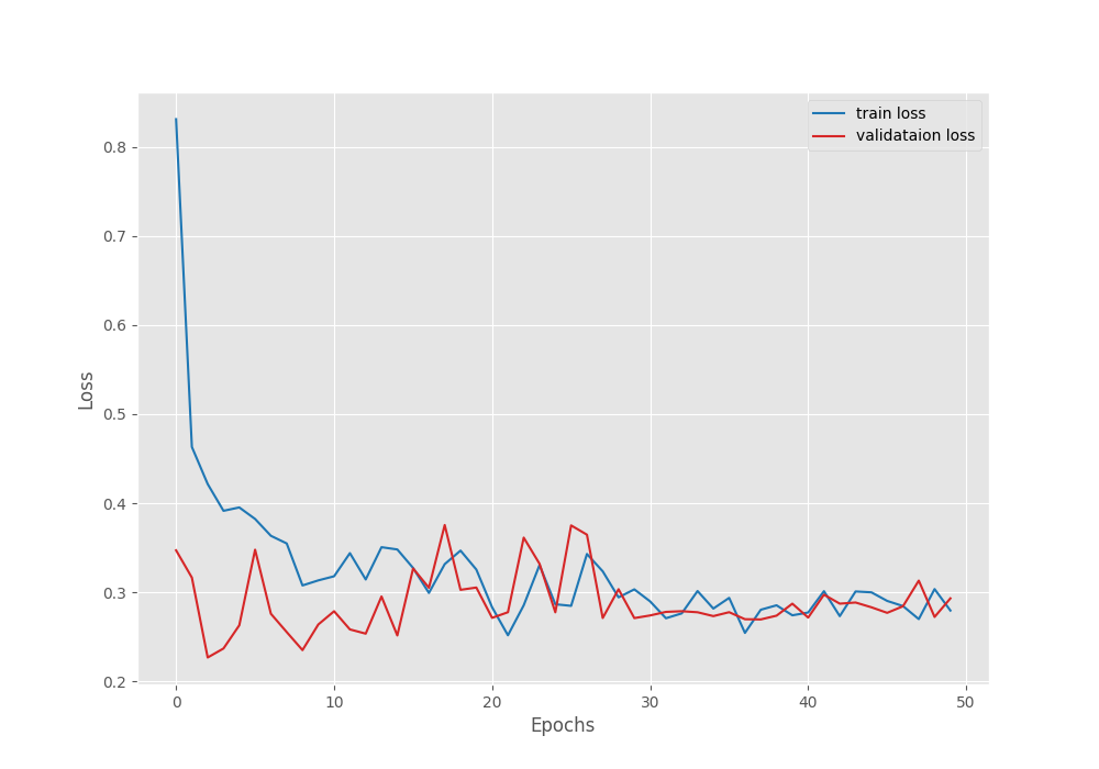
The validation loss seems to be stabilizing more after 30 epochs when the learning rate scheduler kicks in.

It seems that the pixel accuracy was increasing till the end of training.

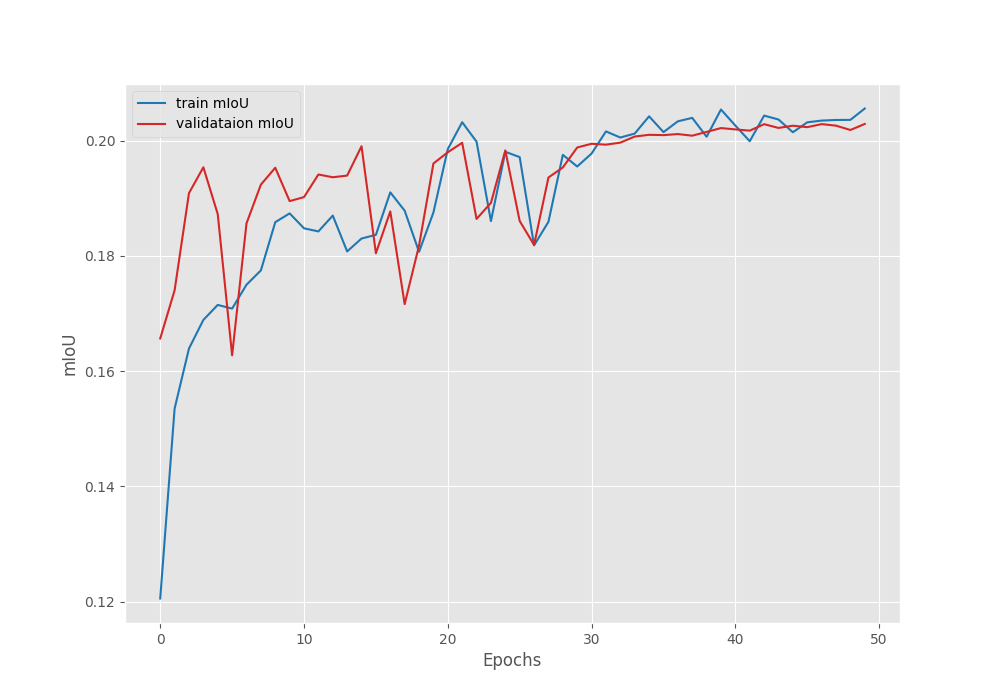
The mIoU plot also seems to be improving till 50 epochs with a few fluctuations. There is a chance that it may further increase if we train for longer.

For now, we have the models with us. Let’s move on to running inference on images and videos.

Inference on Images

All the inference experiments were run on a laptop with GTX 1060 GPU, 16 GB RAM, and 8th gen i7 processor.

For running inference on images, we will use the infer_image.py script. It accepts the following command line arguments.

• --input: The path to the directory containing images.
• --device: It is the computation device. This defaults to the CUDA device.
• --imgsz: This accepts two values, one for width and one for height. If we do not provide anything, then the inference will be run on the original image resolution.
• --model: Path to the model directory. It defaults to outputs/model_iou.

Let’s run inference on the validation images from the Pascal VOC dataset.

python infer_image.py --input input/voc_2012_segmentation_data/valid_images/

Here are some of the results.

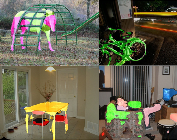
It is clear that the model is performing the best when segmenting humans. For other objects, like bicycles, or animals, the segmentation maps are not precise. This is mostly because we had 20 object classes and around 1400 training images only.

Still, this goes a long way to show that by using SegFormer we achieve more than decent results even on a small dataset.

Inference on Videos

We will run the infer_video.py script for running inference on videos. All the command line arguments remain the same with the exception that --input now accepts the path to a video file.

Let’s start with a simple video where we have people in the scene.

python infer_video.py --input input/inference_data/videos/video_1.mp4

The segmentation maps are very precise when the whole body of the person is visible.

Now, let’s run inference where a person and dogs are present.

python infer_video.py --input input/inference_data/videos/video_2.mp4

In some of the scenes, the mode is segmenting the dog as another object. Else, the predictions look nice.

Now, a final video where a person is riding a horse.

python infer_video.py --input input/inference_data/videos/video_3.mp4

The model is able to segment the persons and the horse accurately in almost all the scenes.

The results go a long way to show how the largest SegFormer model is able to perform so well even when the dataset is imbalanced.

Summary and Conclusion

In this blog post, we fine-tuned the SegFormer-B5 model on the Pascal VOC segmentation dataset. Even though the dataset is imbalanced, the inference results showed how well the model performs. This showcases the power of Transformer based models in Computer Vision and Deep Learning. I hope that this article was worth your time.

If you have any doubts, thoughts, or suggestions, please leave them in the comment section. I will surely address them.

You can contact me using the Contact section. You can also find me on LinkedIn, and Twitter.