Fine Tuning Mask2Former

Mask2Former is a universal image segmentation model that uses a single architecture to carry out semantic, instance, and panoptic segmentation. In the previous article, we went through an overview of Mask2Former including its architecture and inference on images & videos. Following that, in this article, we will be fine tuning Mask2Former. We will use a binary segmentation dataset with one background class and one object class with semantic masks. This is a simple problem to start with. However, it will help us understand the entire pipeline for training Mask2Former.

Training Mask2Former can be a rather complex process. There are a few caveats that we need to take care of while preparing the model and dataset. We will cover all these in detail here while trying to get the best out of Mask2Former’s capabilities.

We will cover the following topics in this article

• In the following section, we will start with the description of the dataset. In brief, we will use a leaf disease segmentation dataset here.
• Following that, we will get into the coding part for training Mask2Former.
  • First, we will discuss loading the Mask2FormerImageProcessor & Mask2FormerForUniversalSegmentation model and all the caveats associated with it.
  • Second, is the dataset preparation. This will include using Mask2FormerImageProcessor to preprocess the images as intended for the model and the training pipeline.
  • Third, we will discuss the training and validation functions that are equally important for fine tuning Mask2Former.
• After training, we will run inference using the trained model and analyze the results

The Leaf Disease Segmentation Dataset

We will use a very interesting leaf disease segmentation dataset for fine tuning Mask2Former. It contains just 2 classes, one is the background class, and the other is the disease mask on the leaves.

You can find the dataset here on Kaggle.

Downloading the dataset and extracting its content reveals the following structure.

leaf_disease_segmentation/
├── aug_data
│   ├── train_images [2500 entries exceeds filelimit, not opening dir]
│   ├── train_masks [2500 entries exceeds filelimit, not opening dir]
│   ├── valid_images [440 entries exceeds filelimit, not opening dir]
│   └── valid_masks [440 entries exceeds filelimit, not opening dir]
└── orig_data
    ├── train_images [498 entries exceeds filelimit, not opening dir]
    ├── train_masks [498 entries exceeds filelimit, not opening dir]
    ├── valid_images [90 entries exceeds filelimit, not opening dir]
    └── valid_masks [90 entries exceeds filelimit, not opening dir]

There are two directories, aug_data containing augmented images & masks and orig_data containing the original images & masks.

We will use the content of orig_data and apply augmentations during dataset preparation. There are 498 training samples and 90 validation samples.

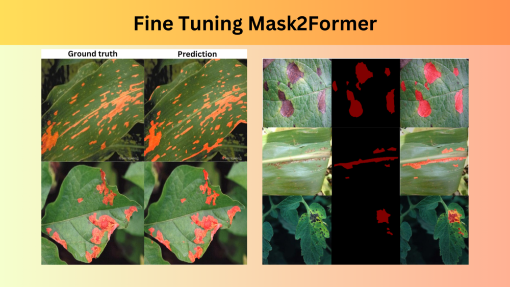
Here are a few examples from the dataset.

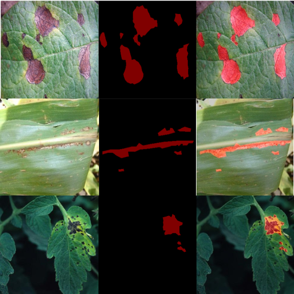
The above figure shows the original image, the original mask, and the mask overlaid on the image. As we can see, the dataset contains masks for different diseases. These include apple scab leaf, apple rust leaf, and bell pepper leaf spot among others.

Project Directory Structure

Let’s take a look at the project directory structure now.

├── input
│   └── leaf_disease_segmentation
│       ├── aug_data
│       └── orig_data
├── outputs
│   ├── final_model
│   │   ├── config.json
│   │   └── model.safetensors
│   ├── inference_results_image [90 entries exceeds filelimit, not opening dir]
│   ├── model_iou
│   │   ├── config.json
│   │   └── model.safetensors
│   ├── model_loss
│   │   ├── config.json
│   │   └── model.safetensors
│   ├── valid_preds [30 entries exceeds filelimit, not opening dir]
│   ├── loss.png
│   └── miou.png
├── config.py
├── custom_datasets.py
├── engine.py
├── infer_image.py
├── infer_video.py
├── model.py
├── train.py
└── utils.py

• The input directory contains the dataset that we discussed earlier.
• The outputs directory contains the trained models, loss & accuracy graphs, and the inference results.
• Finally, the parent project directory contains all the Python code files.

Library Dependencies

We will use the PyTorch framework in this article for training Mask2Former on the binary segmentation dataset. Along with that, we will need the Hugging Face transformers and evaluate libraries.

If you need, you can execute the following commands to install them in the environment of your choice.

PyTorch Installation

conda install pytorch torchvision torchaudio pytorch-cuda=11.8 -c pytorch -c nvidia

Transformers Installation

pip install transformers

Evaluate Installation

pip install evaluate

That’s all the major dependencies for following through this article.

All the Python code files and best trained model will be provided via the ‘Download Code’ section. In case, you wish to run training and inference, you can download and set the data set in the above structure.

Fine Tuning Mask2Former

Let’s get down to the coding part now. We will cover all the necessary code files as required.

Download Code

The Configuration File

First of all, let’s take a look at the configuration file, that is, the config.py Python file.

ALL_CLASSES = ['background', 'disease']

LABEL_COLORS_LIST = [
    (0, 0, 0), # Background.
    (128, 0, 0),
]

VIS_LABEL_MAP = [
    (0, 0, 0), # Background.
    (255, 0, 0),
]

It contains three lists.

• ALL_CLASSES: It contains the name of the segmentation mask classes. For us, it is the background class and the disease class. We can add any relevant name here.
• LABEL_COLORS_LIST: This list contains the color values that each class has been annotated within the dataset. The background annotation is completely black, so it is (0, 0, 0). For the diseased parts’ mask, the color is a hue of red, that is (128, 0, 0).
• VIS_LABEL_MAP: This list contains the color that we want to visualize the masks with during inference. In most cases, keeping it the same as the LABEL_COLORS_LIST works the best. However, in this case, we change the disease masks to a brighter red color for better visualizations.

Loading the Mask2Former Model and The Mask2Former Image Processor

Both, the Mask2Former model and the Image Processor are crucial parts of the training pipeline. Initializing them properly is important. We load the model and the image processor in the next code block and this content goes into the model.py file.

from transformers import (
    Mask2FormerForUniversalSegmentation, Mask2FormerImageProcessor
)

def load_model(num_classes=1):
    image_processor = Mask2FormerImageProcessor(
        ignore_index=255, reduce_labels=True
    )

    model = Mask2FormerForUniversalSegmentation.from_pretrained(
        'facebook/mask2former-swin-tiny-ade-semantic',
        num_labels=num_classes,
        ignore_mismatched_sizes=True
    )

    return model, image_processor

We import two classes in the above code block, Mask2FormerForUniversalSegmentation and Mask2FormerImageProcessor. The former is for loading the model and the latter is for loading the image processor.

The load_model function accepts a single parameter defining the number of classes in the dataset. Inside the function, first, we load the Mask2FormerImageProcessor while passing the ignore_index and reduce_labels parameters.

The image_processor helps preprocess all the input images and masks to the required format for training the Mask2Former model.

The ignore_index parameter defines a label number that we do not have in the dataset and would like the loss function to ignore. As we just have two classes, so, the first label is 0 and the second one is 1. Therefore, we pass 255 to the parameter. The second parameter is reduce_labels which accepts a boolean value and we pass True. This will reduce all labels in our dataset by 1.

A question arises here. What would happen if we pass the default values to them, None and False respectively. In that case, we get a very specific runtime error.

ValueError: Unsupported format: None

And this happens while padding the mask which is a function of the image processing class. Only by providing a combination of the arguments as shown in the earlier code block, we can train the model successfully and properly visualize the masks during inference. At the time of writing this article, I have not been able to find a justification for this. But mostly, it seems like how the code handles padding values, as they are 0s by default in image processing. And therefore, having a 0 labeled class in the dataset is causing issues.

The Dataset Preparation

The dataset preparation is equally important for any segmentation project. We will handle a few important things here as well. The code for this resides in the custom_datasets.py file.

Let’s start with the imports, defining necessary constants, and the data transforms.

import glob
import albumentations as A
import cv2
import numpy as np

from utils import get_label_mask, set_class_values
from torch.utils.data import Dataset, DataLoader
from functools import partial

# ADE data mean and standard deviation.
ADE_MEAN = np.array([123.675, 116.280, 103.530]) / 255
ADE_STD = np.array([58.395, 57.120, 57.375]) / 255

def get_images(root_path):
    train_images = glob.glob(f"{root_path}/train_images/*")
    train_images.sort()
    train_masks = glob.glob(f"{root_path}/train_masks/*")
    train_masks.sort()
    valid_images = glob.glob(f"{root_path}/valid_images/*")
    valid_images.sort()
    valid_masks = glob.glob(f"{root_path}/valid_masks/*")
    valid_masks.sort()

    return train_images, train_masks, valid_images, valid_masks

def train_transforms(img_size):
    """
    Transforms/augmentations for training images and masks.

    :param img_size: Integer, for image resize.
    """
    train_image_transform = A.Compose([
        A.Resize(img_size[1], img_size[0], always_apply=True),
        A.HorizontalFlip(p=0.5),
        A.RandomBrightnessContrast(p=0.25),
        A.Rotate(limit=25),
        A.Normalize(mean=ADE_MEAN, std=ADE_STD)
    ], is_check_shapes=False)
    return train_image_transform

def valid_transforms(img_size):
    """
    Transforms/augmentations for validation images and masks.

    :param img_size: Integer, for image resize.
    """
    valid_image_transform = A.Compose([
        A.Resize(img_size[1], img_size[0], always_apply=True),
        A.Normalize(mean=ADE_MEAN, std=ADE_STD)
    ], is_check_shapes=False)
    return valid_image_transform

As you may have observed in the model loading section, we are using the Mask2Former tiny model pretrained on the ADE20K dataset. To get the best possible results, normalization values should also match. For this reason, we are using the ADE20K dataset’s mean and standard deviation values for normalizing the input images here.

The train_transforms function defines the image processing and augmentations that we apply to the training set. These include resizing the images and masks, and image augmentation like:

• Horizontal flipping
• Randomizing brightness and contrast
• Rotating the images and masks

For the validation set, we just resize the samples and apply the normalization.

The next block of code is crucial.

def collate_fn(batch, image_processor):
    inputs = list(zip(*batch))
    images = inputs[0]
    segmentation_maps = inputs[1]

    batch = image_processor(
        images,
        segmentation_maps=segmentation_maps,
        return_tensors='pt',
        do_resize=False,
        do_rescale=False,
        do_normalize=False
    )

    batch['orig_image'] = inputs[2]
    batch['orig_mask'] = inputs[3]
    return batch

class SegmentationDataset(Dataset):
    def __init__(
        self, 
        image_paths, 
        mask_paths, 
        tfms, 
        label_colors_list,
        classes_to_train,
        all_classes,
        feature_extractor
    ):
        self.image_paths = image_paths
        self.mask_paths = mask_paths
        self.tfms = tfms
        self.label_colors_list = label_colors_list
        self.all_classes = all_classes
        self.classes_to_train = classes_to_train
        self.class_values = set_class_values(
            self.all_classes, self.classes_to_train
        )
        self.feature_extractor = feature_extractor

    def __len__(self):
        return len(self.image_paths)

    def __getitem__(self, index):
        image = cv2.imread(self.image_paths[index], cv2.IMREAD_COLOR)
        image = cv2.cvtColor(image, cv2.COLOR_BGR2RGB).astype('uint8')
        mask = cv2.imread(self.mask_paths[index], cv2.IMREAD_COLOR)
        mask = cv2.cvtColor(mask, cv2.COLOR_BGR2RGB).astype('float32')

        transformed = self.tfms(image=image, mask=mask)
        image = transformed['image']
        orig_image = image.copy()
        image = image.transpose(2, 0, 1)
        mask = transformed['mask']
        
        # Get 2D label mask.
        mask = get_label_mask(mask, self.class_values, self.label_colors_list)
        orig_mask = mask.copy()
        
        return image, mask, orig_image, orig_mask

First, we have the collate_fn function. It accepts a batch of images and the image processor as parameters.

The batch variable is a tuple containing four values that we get from the dataset class. They are the transformed images, the 2D masks, and the original images and masks.

First, we convert them into a list of tuples and pass them through the Mask2Former image processor. The first argument accepts the images, and the second one the segmentation maps. Apart from that, we also pass the following arguments.

• return_tensors='pt': To get back tensors in PyTorch acceptable format.
• do_resize=False, do_rescale=False, do_normalize=False: As we are handling all of this on our own during the Albumentation transformation phase.

After we obtain the batches (a dictionary), we add the original image and mask values with new keys. As we will see later on, we need them during the training and validation phase.

Finally, we prepare the datasets and data loaders.

def get_dataset(
    train_image_paths, 
    train_mask_paths,
    valid_image_paths,
    valid_mask_paths,
    all_classes,
    classes_to_train,
    label_colors_list,
    img_size,
    feature_extractor
):
    train_tfms = train_transforms(img_size)
    valid_tfms = valid_transforms(img_size)

    train_dataset = SegmentationDataset(
        train_image_paths,
        train_mask_paths,
        train_tfms,
        label_colors_list,
        classes_to_train,
        all_classes, 
        feature_extractor
    )
    valid_dataset = SegmentationDataset(
        valid_image_paths,
        valid_mask_paths,
        valid_tfms,
        label_colors_list,
        classes_to_train,
        all_classes,
        feature_extractor
    )
    return train_dataset, valid_dataset

def get_data_loaders(train_dataset, valid_dataset, batch_size, processor):
    collate_func = partial(collate_fn, image_processor=processor)

    train_data_loader = DataLoader(
        train_dataset, 
        batch_size=batch_size, 
        drop_last=False, 
        num_workers=8,
        shuffle=True,
        collate_fn=collate_func
    )
    valid_data_loader = DataLoader(
        valid_dataset, 
        batch_size=batch_size, 
        drop_last=False, 
        num_workers=8,
        shuffle=False,
        collate_fn=collate_func
    )

    return train_data_loader, valid_data_loader  

For the data loaders, we are using 8 parallel workers. You can adjust the value according to your hardware configuration.

The Training and Validation Function

The training and validation functions reside in the engine.py file. For fine tuning Mask2Former, they are just as crucial. First, we have the import statements.

import torch
import torch.nn.functional as F

from tqdm import tqdm
from utils import draw_translucent_seg_maps

We are importing one draw_transluscent_seg_maps function from the utils module. During validation, it saves an image from the validation set with the predicted segmentation map overlaid on it. This helps analyze the model’s progress qualitatively after each epoch.

Now, coming to the training function.

def train(
    model,
    train_dataloader,
    device,
    optimizer,
    classes_to_train,
    processor,
    metric
):
    print('Training')
    model.train()
    train_running_loss = 0.0
    prog_bar = tqdm(
        train_dataloader, 
        total=len(train_dataloader), 
        bar_format='{l_bar}{bar:20}{r_bar}{bar:-20b}'
    )
    counter = 0 # to keep track of batch counter
    num_classes = len(classes_to_train)

    for i, data in enumerate(prog_bar):
        counter += 1

        pixel_values = data['pixel_values'].to(device)
        mask_labels = [mask_label.to(device) for mask_label in data['mask_labels']]
        class_labels = [class_label.to(device) for class_label in data['class_labels']]
        pixel_mask = data['pixel_mask'].to(device)

        optimizer.zero_grad()
        outputs = model(
            pixel_values=pixel_values, 
            mask_labels=mask_labels,
            class_labels=class_labels,
            pixel_mask=pixel_mask
        )

        ##### BATCH-WISE LOSS #####
        loss = outputs.loss
        train_running_loss += loss.item()
        ###########################
 
        ##### BACKPROPAGATION AND PARAMETER UPDATION #####
        loss.backward()
        optimizer.step()
        ##################################################

        target_sizes = [(image.shape[0], image.shape[1]) for image in data['orig_image']]
        pred_maps = processor.post_process_semantic_segmentation(
            outputs, target_sizes=target_sizes
        )

        metric.add_batch(references=data['orig_mask'], predictions=pred_maps)
        
    ##### PER EPOCH LOSS #####
    train_loss = train_running_loss / counter
    ##########################
    iou = metric.compute(num_labels=num_classes, ignore_index=255, reduce_labels=True)['mean_iou']
    return train_loss, iou

The function accepts the model, training data loader, computation device, optimizer, the classes we want to train, image processor, and the metric as parameters.

The metric is initialized through the evaluate library for computing IoU value as we will see in the training script.

Let’s get down to the iteration starting from line number 21.

A batch of data from the data loader is holding the following 4 values.

• pixel_values and mask_labels: The former is the preprocessed images in the batch and the latter is a list containing binary masks for each segmented object in that batch.
• class_labels: This is a list of tensors containing the label indexes for each sample in the mask_labels. For example, if there are two samples (batch size of 2), then class_labels will be [tensor([0, 1]), tensor([0, 1])].
• pixel_mask: This is a converted mask where the shape is [batch_size, height, width].

The model accepts all four values in the forward pass and gives us the outputs dictionary. We can directly extract the loss from it and use it for backpropagation.

But we also need to compute the IoU (Intersection over Union). For this, we use the image processors’ post_process_semantic_segmentation to obtain the resulting 2D masks and pass them along with the original masks to the metrics’ add_batch function.

Finally, we return the epoch’s loss and IoU values.

The validation function is almost similar with slight variations.

def validate(
    model,
    valid_dataloader,
    device,
    classes_to_train,
    label_colors_list,
    epoch,
    save_dir,
    processor,
    metric
):
    print('Validating')
    model.eval()
    valid_running_loss = 0.0
    num_classes = len(classes_to_train)

    with torch.no_grad():
        prog_bar = tqdm(
            valid_dataloader, 
            total=(len(valid_dataloader)), 
            bar_format='{l_bar}{bar:20}{r_bar}{bar:-20b}'
        )
        counter = 0 # To keep track of batch counter.
        for i, data in enumerate(prog_bar):
            counter += 1

            pixel_values = data['pixel_values'].to(device)
            mask_labels = [mask_label.to(device) for mask_label in data['mask_labels']]
            class_labels = [class_label.to(device) for class_label in data['class_labels']]
            pixel_mask = data['pixel_mask'].to(device)

            outputs = model(
                pixel_values=pixel_values, 
                mask_labels=mask_labels,
                class_labels=class_labels,
                pixel_mask=pixel_mask
            )

            target_sizes = [(image.shape[0], image.shape[1]) for image in data['orig_image']]
            pred_maps = processor.post_process_semantic_segmentation(
                outputs, target_sizes=target_sizes
            )
                
            # Save the validation segmentation maps.
            if i == 0:
                draw_translucent_seg_maps(
                    pixel_values, 
                    pred_maps, 
                    epoch, 
                    i, 
                    save_dir, 
                    label_colors_list,
                )

            ##### BATCH-WISE LOSS #####
            loss = outputs.loss
            valid_running_loss += loss.item()
            ###########################

            metric.add_batch(references=data['orig_mask'], predictions=pred_maps)
        
    ##### PER EPOCH LOSS #####
    valid_loss = valid_running_loss / counter
    ##########################
    iou = metric.compute(num_labels=num_classes, ignore_index=255, reduce_labels=True)['mean_iou']
    return valid_loss, iou

As we can see on line 108, we save one image from the first batch with its predicted segmentation map using the draw_translucent_seg_maps function.

There is one more important point to note in both functions. For the IoU calculation, we are passing ignore_index=255 and reduce_labels=True just like we did with the image processor. This ensures the correct calculation of the IoU.

The Training Script for Mask2Former

The code to train the Mask2Former model is in the train.py file.

Let’s go through the imports and the argument parsers first.

import torch
import os
import argparse
import evaluate

from custom_datasets import get_images, get_dataset, get_data_loaders
from model import load_model
from config import ALL_CLASSES, LABEL_COLORS_LIST
from engine import train, validate
from utils import save_model, SaveBestModel, save_plots, SaveBestModelIOU
from torch.optim.lr_scheduler import MultiStepLR

seed = 42
torch.manual_seed(seed)
torch.cuda.manual_seed(seed)
torch.backends.cudnn.deterministic = True
torch.backends.cudnn.benchmark = True

parser = argparse.ArgumentParser()
parser.add_argument(
    '--epochs',
    default=10,
    help='number of epochs to train for',
    type=int
)
parser.add_argument(
    '--lr',
    default=0.0001,
    help='learning rate for optimizer',
    type=float
)
parser.add_argument(
    '--batch',
    default=4,
    help='batch size for data loader',
    type=int
)
parser.add_argument(
    '--imgsz', 
    default=[512, 512],
    type=int,
    nargs='+',
    help='width, height'
)
parser.add_argument(
    '--scheduler',
    action='store_true',
)
parser.add_argument(
    '--scheduler-epochs',
    dest='scheduler_epochs',
    default=[50],
    nargs='+',
    type=int
)
args = parser.parse_args()
print(args)

We import all the necessary libraries and custom modules. Along with that, we set the seed for deterministic runs, and define the command line arguments.

Following is the main code block.

if __name__ == '__main__':
    # Create a directory with the model name for outputs.
    out_dir = os.path.join('outputs')
    out_dir_valid_preds = os.path.join(out_dir, 'valid_preds')
    os.makedirs(out_dir, exist_ok=True)
    os.makedirs(out_dir_valid_preds, exist_ok=True)

    device = torch.device('cuda:0' if torch.cuda.is_available() else 'cpu')
    model, processor = load_model(num_classes=len(ALL_CLASSES))
    model = model.to(device)
    print(model)
    # Total parameters and trainable parameters.
    total_params = sum(p.numel() for p in model.parameters())
    print(f"{total_params:,} total parameters.")
    total_trainable_params = sum(
        p.numel() for p in model.parameters() if p.requires_grad)
    print(f"{total_trainable_params:,} training parameters.")

    optimizer = torch.optim.AdamW(model.parameters(), lr=args.lr)

    train_images, train_masks, valid_images, valid_masks = get_images(
        root_path='input/leaf_disease_segmentation/orig_data'    
    )

    train_dataset, valid_dataset = get_dataset(
        train_images, 
        train_masks,
        valid_images,
        valid_masks,
        ALL_CLASSES,
        ALL_CLASSES,
        LABEL_COLORS_LIST,
        img_size=args.imgsz,
        feature_extractor=processor
    )

    train_dataloader, valid_dataloader = get_data_loaders(
        train_dataset, 
        valid_dataset,
        args.batch,
        processor
    )

    # Initialize `SaveBestModel` class.
    save_best_model = SaveBestModel()
    save_best_iou = SaveBestModelIOU()
    # LR Scheduler.
    scheduler = MultiStepLR(
        optimizer, milestones=args.scheduler_epochs, gamma=0.1, verbose=True
    )

    train_loss, train_miou = [], []
    valid_loss, valid_miou = [], []
    
    metric = evaluate.load("mean_iou")

    for epoch in range (args.epochs):
        print(f"EPOCH: {epoch + 1}")
        train_epoch_loss, train_epoch_miou = train(
            model,
            train_dataloader,
            device,
            optimizer,
            ALL_CLASSES,
            processor,
            metric
        )
        valid_epoch_loss, valid_epoch_miou = validate(
            model,
            valid_dataloader,
            device,
            ALL_CLASSES,
            LABEL_COLORS_LIST,
            epoch,
            save_dir=out_dir_valid_preds,
            processor=processor,
            metric=metric
        )
        train_loss.append(train_epoch_loss)
        # train_pix_acc.append(train_epoch_pixacc)
        train_miou.append(train_epoch_miou)
        valid_loss.append(valid_epoch_loss)
        # valid_pix_acc.append(valid_epoch_pixacc)
        valid_miou.append(valid_epoch_miou)

        save_best_model(
            valid_epoch_loss, epoch, model, out_dir, name='model_loss'
        )
        save_best_iou(
            valid_epoch_miou, epoch, model, out_dir, name='model_iou'
        )

        print(
            f"Train Epoch Loss: {train_epoch_loss:.4f},",
            f"Train Epoch mIOU: {train_epoch_miou:4f}"
        )
        print(
            f"Valid Epoch Loss: {valid_epoch_loss:.4f},", 
            f"Valid Epoch mIOU: {valid_epoch_miou:4f}"
        )
        if args.scheduler:
            scheduler.step()
        print('-' * 50)

    # Save the loss and accuracy plots.
    save_plots(
        train_loss, valid_loss,
        train_miou, valid_miou, 
        out_dir
    )
    # Save final model.
    save_model(model, out_dir, name='final_model')
    print('TRAINING COMPLETE')

This combines everything we have covered till now. Starting from the data loaders, the optimizer, to the metric. After every epoch, we try to save the best model based on the current validation loss and validation IoU.

Other than this, the utils.py file contains a few helper functions and classes. These include functions to save the loss and IoU graphs, for saving the model, and even for creating the overlaid images using the predicted segmentation maps. You may go through them if you are interested.

Executing train.py and Fine Tuning Mask2Former

Let’s execute the training script to start the fine tuning process. The training and inference shown here were carried out on a machine with 10 GB RTX 3080 GPU, i7 10th generation CPU, and 32 GB RAM.

python train.py --imgsz 320 320 --epochs 30 --lr 0.0001 --batch 10

We are training the Mask2Former model for 30 epochs with an image size of 320×320, a learning rate of 0.0001, and a batch size of 10.

Following are the output logs from the final few epochs.

EPOCH: 29
Training
100%|████████████████████| 50/50 [04:12<00:00,  5.06s/it]                                                                                                                                                          
Validating
100%|████████████████████| 9/9 [00:22<00:00,  2.49s/it]                                                                                                                                                            

Best validation IoU: 0.867643805173509

Saving best model for epoch: 29

Train Epoch Loss: 14.5157, Train Epoch mIOU: 0.936340
Valid Epoch Loss: 24.0145, Valid Epoch mIOU: 0.867644
--------------------------------------------------
EPOCH: 30
Training
100%|████████████████████| 50/50 [04:10<00:00,  5.01s/it]                                                                                                                                                          
Validating
100%|████████████████████| 9/9 [00:22<00:00,  2.54s/it]                                                                                                                                                            

Best validation loss: 22.748868730333115

Saving best model for epoch: 30

Train Epoch Loss: 14.6232, Train Epoch mIOU: 0.932732
Valid Epoch Loss: 22.7489, Valid Epoch mIOU: 0.865820
--------------------------------------------------
TRAINING COMPLETE

The model reached its best validation IoU of 86.76% on epoch 29 and the best validation loss of 22.74 on the last epoch. We can observe that the loss values are higher than what we typically see in deep learning based computer vision model training. However, it seems that the model is learning and it is mostly a quirk of the Mask2Former model.

Let’s take a look at the IoU and loss graphs to gain more insight.

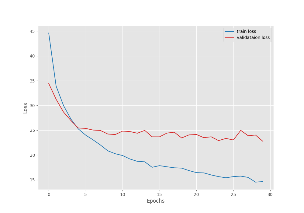
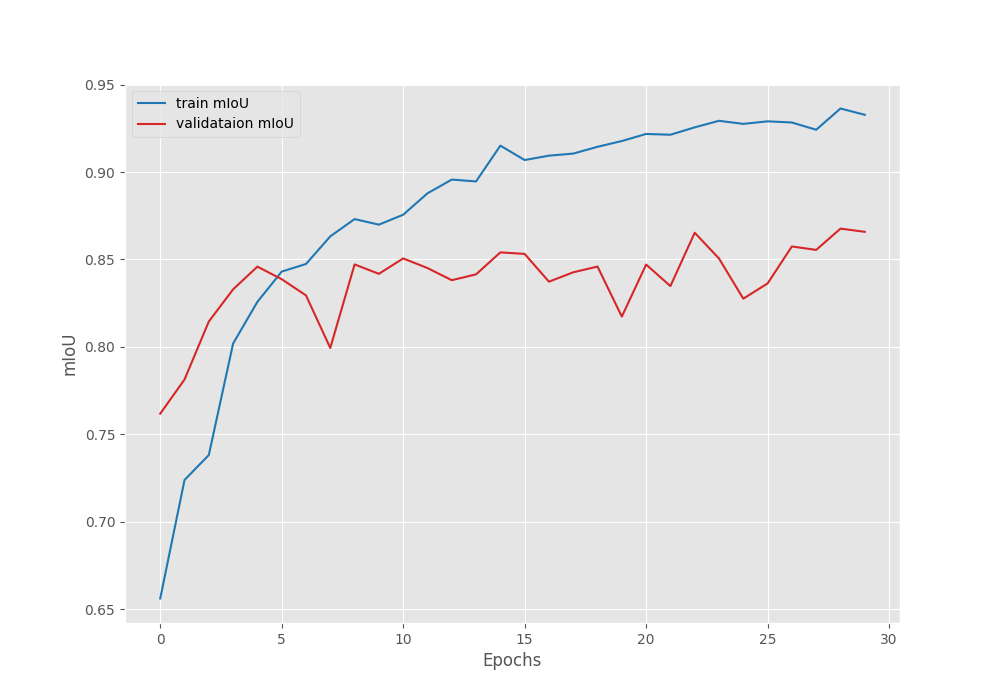
Both, the loss graph and IoU graph seem to be improving till the end of training. Most probably, we can train the model for even longer to achieve even better results. However, for now, we have a good model with us and can move to the inference part.

Inference using the Trained Mask2Former Model

For inference, we will use the weights saved according to the best IoU and check the results on the validation images from the dataset.

The infer_image.py file contains the code for running inference on images.

Following are the import statements and argument parsers for the script.

from transformers import (
    Mask2FormerForUniversalSegmentation, Mask2FormerImageProcessor
)
from config import VIS_LABEL_MAP as LABEL_COLORS_LIST
from utils import (
    draw_segmentation_map, 
    image_overlay,
    predict
)

import argparse
import cv2
import os
import glob

parser = argparse.ArgumentParser()
parser.add_argument(
    '--input',
    help='path to the input image directory',
    default='input/inference_data/images'
)
parser.add_argument(
    '--device',
    default='cuda:0',
    help='compute device, cpu or cuda'
)
parser.add_argument(
    '--imgsz', 
    default=None,
    type=int,
    nargs='+',
    help='width, height'
)
parser.add_argument(
    '--model',
    default='outputs/model_iou'
)
args = parser.parse_args()

out_dir = 'outputs/inference_results_image'
os.makedirs(out_dir, exist_ok=True)

We import the VIS_LABEL_MAP which contains the RGB color list that we will use for overlaying the segmentation map on the image. From the utils module, we import the predict function. It carries out the forward pass through the model and returns the final 2D segmentation map. It is very similar to what we did in the previous article when carrying out inference using Mask2Former.

The --input argument accepts a directory of images, --device is the computation device, and the --imgsz for passing the image width and height for resizing. By default, the script uses the model with the best IoU.

Next, we need to define the Mask2Former image processor and load the pretrained model. Along with that, we will loop over each image path and carry out the inference.

processor = Mask2FormerImageProcessor()
model = Mask2FormerForUniversalSegmentation.from_pretrained(args.model)
model.to(args.device).eval()

image_paths = glob.glob(os.path.join(args.input, '*'))
for image_path in image_paths:
    image = cv2.imread(image_path)
    if args.imgsz is not None:
        image = cv2.resize(image, (args.imgsz[0], args.imgsz[1]))
    image = cv2.cvtColor(image, cv2.COLOR_BGR2RGB)
    
    # Get labels.
    labels = predict(model, processor, image, args.device)
    
    # Get segmentation map.
    seg_map = draw_segmentation_map(
        labels.cpu(), LABEL_COLORS_LIST
    )
    outputs = image_overlay(image, seg_map)
    cv2.imshow('Image', outputs)
    cv2.waitKey(1)
    
    # Save path.
    image_name = image_path.split(os.path.sep)[-1]
    save_path = os.path.join(
        out_dir, image_name
    )
    cv2.imwrite(save_path, outputs)

After we obtain the 2D labels (line 54), the draw_segmentation_map function generates the RGB segmentation map and the image_overlay function returns the final image with the RGB segmentation map overlaid on the image.

Let’s execute the script and analyze the results.

python infer_image.py --input input/leaf_disease_segmentation/orig_data/valid_images/ --imgsz 320 320

Here are some of the good results that we obtained from the model.

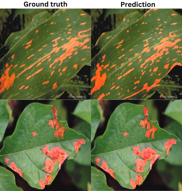
As we can see, the results in the above cases are very accurate.

The following figure shows a few samples where the model did not perform well.

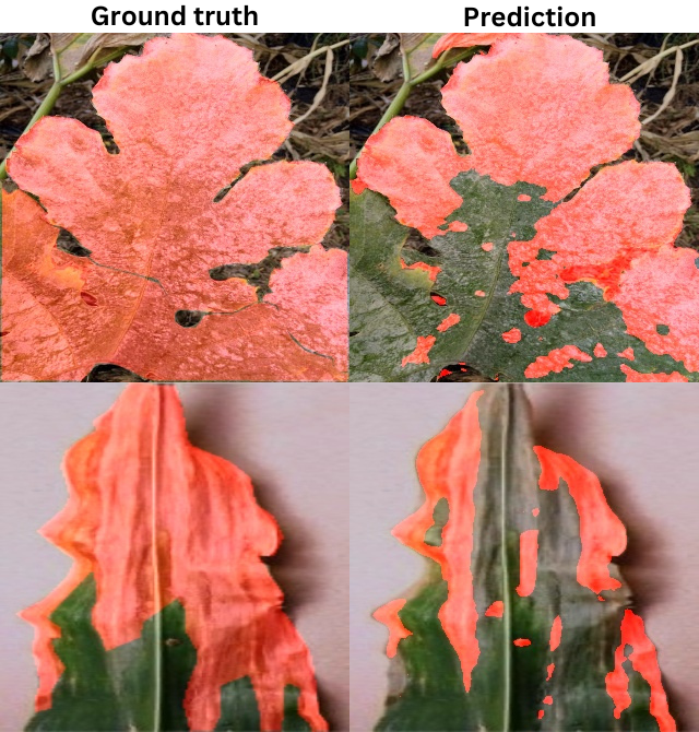
The above are a few samples where the model will perform well if trained for longer.

Summary and Conclusion

We fine tuned the Mask2Former model in this article. While doing so, we went through the dataset preparation, the intricacies related to Mask2Former’s image processing, and the training & inference. In future articles, we will try to train the Mask2Former model on a more diverse and multi-class segmentation dataset. I hope that this article was worth your time.

If you have any doubts, thoughts, or suggestions, please leave them in the comment section. I will surely address them.

You can contact me using the Contact section. You can also find me on LinkedIn, and Twitter.