
SUNet or Swin Transformer UNet for Image Denoising is a Transformer based model for image denoising. Image denoising and image restoration is a field where mostly CNN based models performed well in the recent past. However, like other fields of computer vision, Transformers are also helping in image denoising. In this blog post, we will discuss the SUNet paper and how it tackles the problem of image denoising. Along with that, we will also run inference using the code provided in the official GitHub repository.
Although there are several state of the art works now for image denoising using Transformers, Swin Transformer models seem to dominate the field. This blog post will work as an introduction to using Swin Transformer for Image Denoising.
What will we cover here?
- We will start with the discussion of the paper. This will include:
- The problem that the SUNet paper tries to solve.
- The architecture of the SUNet model.
- Training criteria of SUNet and the results.
- After discussing the paper, we will get hands-on by running inference for image denoising using the pretrained SUNet model.
SUNet for Image Denoising
Due to their impressive performance in image classification, object detection, and segmentation, it was inevitable that Swin Transformers also entered the field of image denoising.
This gave rise to SUNet, a Swin Transformer based UNet model for Image Denoising. The authors of the paper are Chi-Mao Fan, Tsung-Jung Liu, and Kuan-Hsien Liu.
Interestingly, the SUNet model for image denoising does not use an entirely Transformer based approach. Instead, it is a hybrid of Convolution and Transformer based models which leads to such impressive results. More on this when discussing the architecture.
In short, the SUNet model uses the Swin Transformer as the basic block with a UNet like architecture.
Contributions of SUNet to the Field of Image Denoising
There are several state of the art models (mostly CNNs) for image denoising. However, the following points make SUNet stand out here:
- Firstly, SUNet is a hybrid model containing both Swin Transformer and UNet.
- Secondly, it uses a dual upsample method to avoid checkerboard artifacts.
- Thirdly, it beats previous CNN based methods on two well known benchmark datasets.
Further, CNNs face issues when dealing with larger patches and modeling long-range dependencies in image denoising. A hybrid model like SUNet seems to tackle the issue very well.
The SUNet Architecture
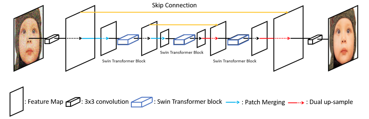
The SUNet model takes inspiration from both Transformer and CNN models. In particular, it is a combination of Swin Transformer and the famous UNet model. However it is important to note that the the UNet structure is built using Swin Transformer blocks and not through CNN blocks.
In summary:
- The image first passes through a 3×3 convolutional layer in the SUNet model to get the initial feature maps.
- These feature maps pass through the main Swin Transformer UNet that provides us with high-level semantic information.
- Finally, a 3×3 convolution reconstructs the denoised image.
Overall, the SUNet model consists of a shallow feature extractor (CNN block), a semantic feature extractor (Swin UNet), and a reconstruction module (CNN block).
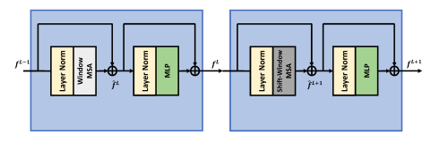
The authors call the Swin Transformer UNet the Swin Transformer Block (STB).
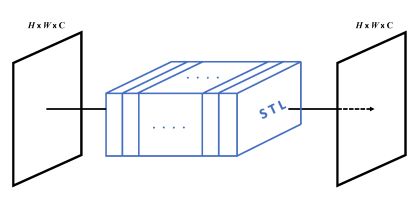
In the final model, the Swin Transformer Block contains 8 Swin Transformer Layers (STL).
For denoising optimization, SUNet uses the very simple L1 pixel loss.
\(\mathcal{L}_{denoise} = ||\hat{X} – X||_1\)
Upsampling Method of SUNet
Image denoising and image restoration in generation can face checkerboard artifacts in the final resulting image. To prevent this, the authors of SUNet use a dual upsampling method. They use:
- The regular bilinar upsampling.
- And also PixelShuffle method.
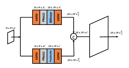
We can see that the feature maps from both the upsampling layers are concatenated along the channel axis.
Training Criteria For SUNet Image Denoising
The SUNet model has been trained on the DIV2K dataset which contains 800 training and 100 validation images. In the data preparation stage, patches are created and gaussian noise is added randomly to the patches with varying level of \(\sigma\) (10, 30, 50). Each patch is of 256×256 spatial resolution.
The entire training takes place on a single NVIDIA GTX 1080Ti GPU. The authors use Peak Signal to Noise Ratio (PSNR) and Image Similarity (SSIM) as the metrics.
Let’s take a look at the resulting table which uses CBSD68 and KODAK24 datasets for evaluation.
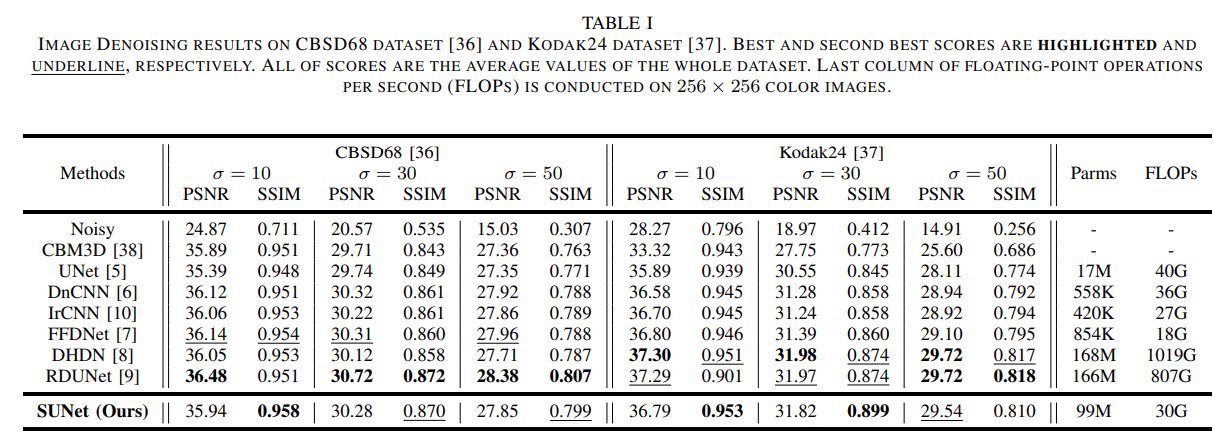
It is evident that the SUNet model does not beat all other models quantitatively. However, with 99 million parameters, it is computationally cheaper compared to the previous state of the art models.
Further, let’s analyze the results qualitatively.
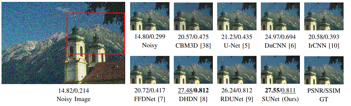
Interestingly, when performing actual image denoising operations, the SUNet model seems to perform extremely well.
Inference using SUNet
Till now, we covered the theoretical and training details of the SUNet model. But getting hands-on with the model will reveal even more. In this section, we will use the official repository and the pretrained model to run inference.
First, we need to clone the SUNet GitHub repository and download the pretrained model.
git clone https://github.com/FanChiMao/SUNet.git
Next, enter the cloned SUNet directory, and download the model directly into it using the following link.
We will be using a simple script to add Gaussian noise to the images. You can download the script and the input images from the following link.
Download the Code
The above link will download an add_noise.py file and a test_images folder containing original and noisy images. Extract the file and copy the files and folders into the cloned SUNet directory.
The final directory structure after copy-pasting the downloaded script, the input image folder, and the pretrained model.
├── datasets
│   ├── DIV2K_noise.m
│   ├── DIV2K_noise_val.m
│   └── README.md
├── model
│   ├── __pycache__
│   ├── SUNet_detail.py
│   └── SUNet.py
├── outputs
│   ├── image_1_256.png
│   ├── image_1.png
│   ├── image_2_256.png
│   ├── image_2.png
│   ├── image_3_256.png
│   └── image_3.png
├── test_images
│   ├── noisy
│   ├── noisy_256
│   └── orig
├── utils
│   ├── __pycache__
│   ├── dataset_utils.py
│   ├── dir_utils.py
│   ├── GaussianBlur.py
│   ├── image_utils.py
│   ├── __init__.py
│   └── model_utils.py
├── warmup_scheduler
│   ├── __pycache__
│   ├── __init__.py
│   ├── run.py
│   └── scheduler.py
├── add_noise.py
├── data_RGB.py
├── dataset_RGB.py
├── demo_any_resolution.py
├── demo.py
├── evaluation.m
├── generate_patches.py
├── model_bestPSNR.pth
├── NOTES.md
├── README.md
├── training.yaml
└── train.py
Adding Gaussian Noise to Images
Although the original and the noisy images are provided with the downloaded zip file, still, let’s go through the procedure of adding Gaussian noise to images.
This is the code in the add_noise.py script.
import cv2
import numpy as np
import glob
import os

def add_gaussian_noise(image, sigma):
    """
    Adds Gaussian noise to an image.

    :param image: Input image to add noise to.
    :param sigma: The standard deviation of the Gaussian noise.

    Returns:
        The noisy image.
    """
    noise = np.random.normal(0, sigma, image.shape)
    noisy_image = image + noise
    return noisy_image
#
if __name__ == '__main__':
    all_images = glob.glob('test_images/orig/*')
    for image_path in all_images:
        np.random.seed(42)
        file_name = image_path.split(os.path.sep)[-1]
        image = cv2.imread(image_path)
        sigma = 15
        noisy_image = add_gaussian_noise(image, sigma)
        if image.shape[:2] == (256, 256):
            cv2.imwrite(f"test_images/noisy_256/{file_name}", noisy_image)
        else:
            cv2.imwrite(f"test_images/noisy/{file_name}", noisy_image)
We simply go over all the images inside test_images/orig directory and add Gaussian noise to each image with a sigma value of 15.
There are both, high resolution images and cropped 256×256 resolution images in the original directory. The high resolution noisy images are stored in the test_images/noisy directory and the cropped images are stored in the test_images/noisy_256 directory. We will get to the reason for this in the next section.
Running Inference
The GitHub repository provides two scripts for running inference.
demo.py: To run inference on 256×256 resolution images.demo_any_resolution.py: To run inference on images of arbitrary resolution.
We will test both scripts here.
SUNet Inference on Arbitrary Image Size
Let’s start with the demo_any_resolution.py script.
python demo_any_resolution.py --input_dir test_images/noisy --weights model_bestPSNR.pth --result_dir outputs
We provide the path to the directory containing the noisy images and the weights file. By default, the images will be stored in the outputs directory.
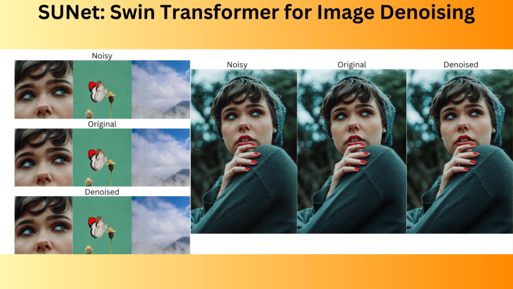
Let’s analyze the images.
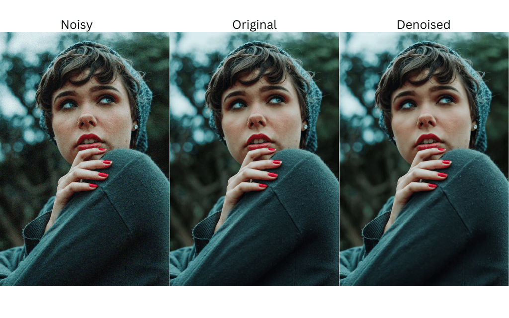
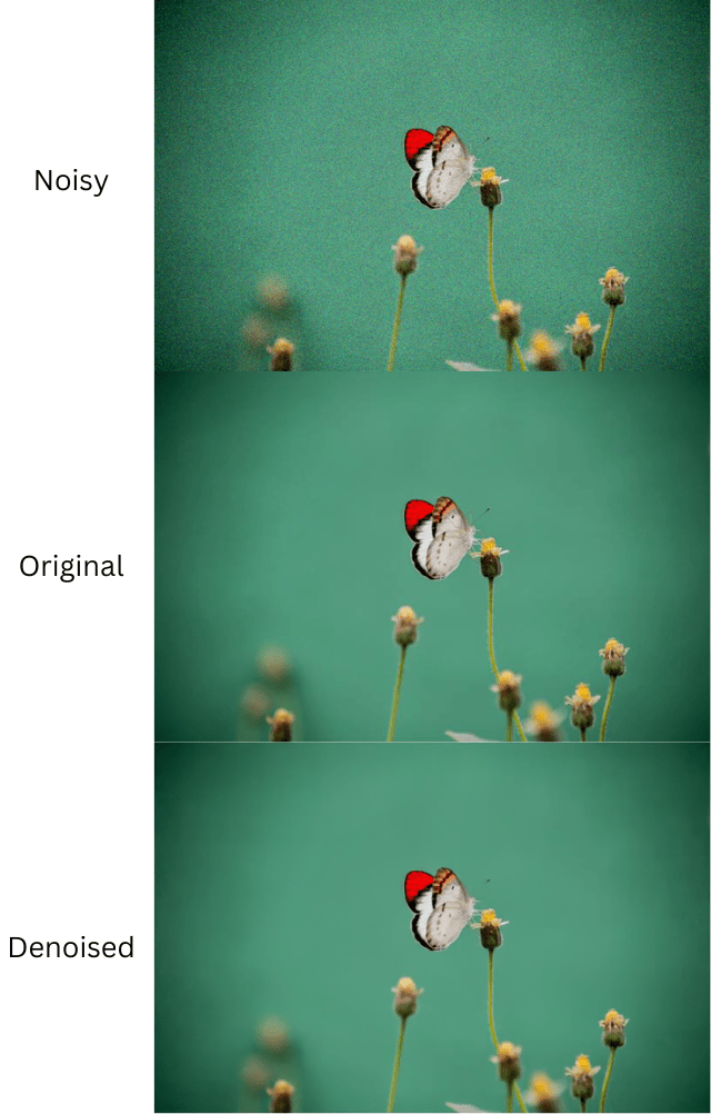
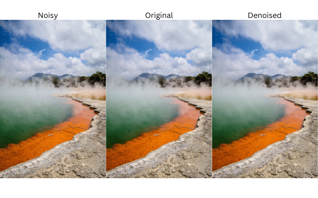
The above figures show the noisy, original, and denoised outputs from the SUNet. The very first thing that we notice is that the images are properly denoised. The SUNet model has done an excellent job here. However, upon closer inspection, we can notice some loss of detail in the denoised outputs. For example, take a look at the face of the woman or the faraway mountains. They look much smoother in the resulting image. This is one of the downsides of noising models today when acting on highly noisy images.
SUNet Inference on Cropped Images
To get an even better idea, let’s work with some cropped images. These cropped ones are from different parts of the above three images.
python demo.py --input_dir test_images/noisy_256/ --weights model_bestPSNR.pth --result_dir outputs
This time, we execute the demo.py script and provide the path to the directory containing the cropped images.
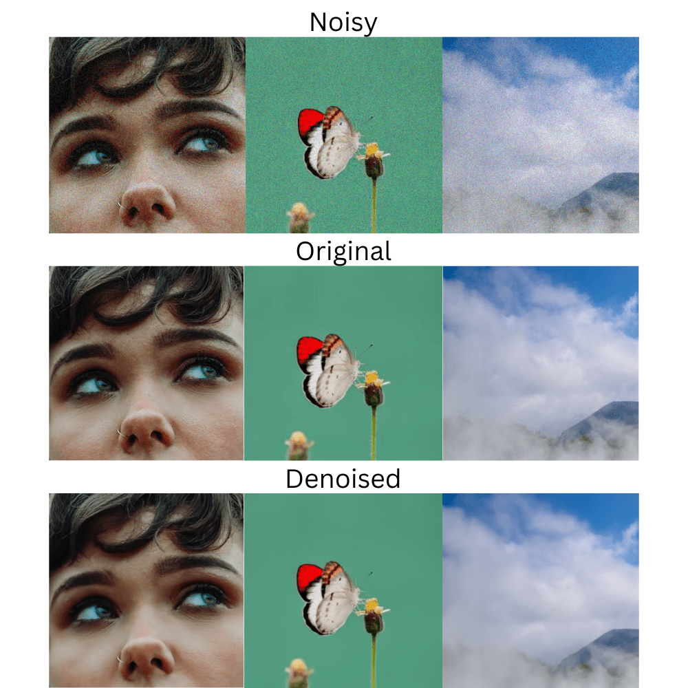
Although the noise is completely gone, with these cropped images, we can clearly see how the resulting image becomes hazy. Of course, when dealing with less noisy images, the final resulting image will be sharper. However, this is something to consider in building future deep learning models for image denoising.
Summary and Conclusion
In this blog post, we discussed the SUNet model for image denoising. The Swin Transformer based UNet model’s architecture, training strategy, and results. We also ran inference which showed the model’s strengths, weaknesses, and where we can improve upon it. I hope this blog post was worth your time.
If you have any doubts, thoughts, or suggestions, please leave them in the comment section. I will surely address them.
You can contact me using the Contact section. You can also find me on LinkedIn, and X.
References
