
In this article, we will implement the Vision Transformer model. Nowadays, it is not absolutely necessary to implement deep learning models from scratch. They are getting bigger and more complex. Understanding the architecture, and their working, and fine-tuning these models will provide similar insights. Still, implementing a model from scratch provides a much deeper understanding of how they work. As such, we will be implementing Vision Transformer from scratch, but not entirely. We will use the torch.nn module which will give us access to the Multi-Head Attention module.
Along with coding from scratch, we will also check whether our implementation matches that of the PyTorch official implementation from Torchvision or not. We can do so by replicating the hyperparameters and checking if the number of trainable parameters matches.
This is the first part of a two-part series. In this article, we will code the Vision Transformer model from scratch. In the next one, we will use the same model and train it from scratch.
Let’s check the topics that we will cover in this article:
- We will start with the implementation of the Vision Transformer model.
- This discussion will include the different parameters that go into the Vision Transformer model and how they affect the final model.
- Also, there are a few caveats that we need to take care of and we will discuss those too.
In the previous post, we have already tried fine-tuning Vision Transformer and visualizing attention maps. Give it a read in case you want to know more about training a Vision Transformer model.
The Directory Structure
The following is the directory structure for the Python file used in this article.
└── model.py
We just have one file. The model.py file contains all the code for creating Vision Transformer from scratch.
Libraries and Dependencies
PyTorch is the only significant dependency for this article.
Coding Vision Transformer from Scratch using torch.nn
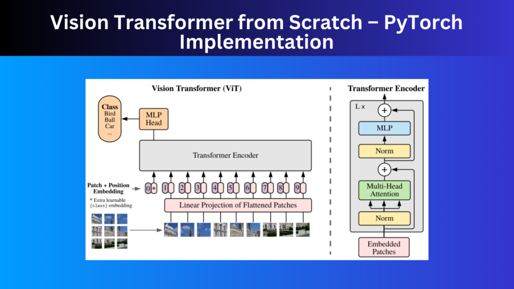
The Vision Transformer model was introduced by Dosovitskiy et al in the paper An Image is Worth 16×16 Words: Transformers for Image Recognition at Scale.
Let’s start coding the Vision Transformer model. As we discussed earlier, it is not entirely from scratch but using the torch.nn module. The major dependency is the MultiheadAttention class that we are not going to code from scratch.
We will go through each section of the model and code. Let’s start with the function that will create patches.
Download Code
2D Convolution to Create Patches
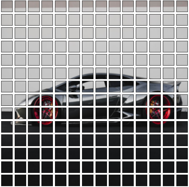
The first and foremost preprocessing step is to convert the images (or more likely tensors) into patches. For instance, take a look at the following image from the paper.

The above is a more simplified version of what happens internally. Suppose that we input 224×224 image (let’s forget about tensors for now) to the patch creation layer. We want each patch to be 16×16 pixels. That would leave us with 224/16 = 14 patches across the height and width.
But do we need to write the patch creation code for Vision Transformer manually? Not necessarily. We can easily employ the nn.Conv2d class for this. The following block creates a CreatePatches class that does the job for us.
import torch.nn as nn
import torch

class CreatePatches(nn.Module):
    def __init__(
        self, channels=3, embed_dim=768, patch_size=16
    ):
        super().__init__()
        self.patch = nn.Conv2d(
            in_channels=channels,
            out_channels=embed_dim,
            kernel_size=patch_size,
            stride=patch_size
        )

    def forward(self, x):
        # Flatten along dim = 2 to maintain channel dimension.
        patches = self.patch(x).flatten(2).transpose(1, 2)
        return patches
So, to create 14 patches across the height and width, we use a kernel_size of 16 and stride of 16. Take note of the patches created in the forward() method. We flatten and transpose the patches. This is because, as we will see later on, apart from this part, we only have Linear layers in the entire Vision Transformer model. So, the flattening of patches becomes mandatory here.
In case, you are wondering, this is what an input tensor that has been encoded, passed through the above class, and decoded again looks like.
One more point to focus on here is the embed_dim (embedding dimension). In Vision Transformers (or most of the transformer neural networks), this is mostly the number of input features that goes into Linear layers.
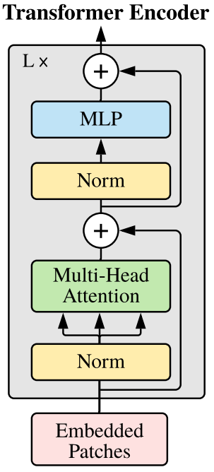
The Self-Attention Block
The next step in creating Vision Transformer from scratch is the Self-Attention block. This is where we will use the MultiheadAttention class from torch.nn.
So, we have the image patches, then they go through some more operations (that we will see later on), which we feed to the Multi-Head Attention module. This is basically a transformer encoder that takes in embeddings and is very similar to what happens in NLP.
Let’s check the code first and then we will go through the explanation.
class AttentionBlock(nn.Module):
    def __init__(self, embed_dim, hidden_dim, num_heads, dropout=0.0):
        super().__init__()

        self.pre_norm = nn.LayerNorm(embed_dim, eps=1e-06)
        self.attention = nn.MultiheadAttention(
            embed_dim=embed_dim,
            num_heads=num_heads,
            dropout=dropout,
            batch_first=True
        )
        self.norm = nn.LayerNorm(embed_dim, eps=1e-06)
        self.MLP = nn.Sequential(
            nn.Linear(embed_dim, hidden_dim),
            nn.GELU(),
            nn.Dropout(dropout),
            nn.Linear(hidden_dim, embed_dim),
            nn.Dropout(dropout)
        )

    def forward(self, x):
        x_norm = self.pre_norm(x)
        # MultiheadAttention returns attention output and weights,
        # we need only the outputs, so [0] index.
        x = x + self.attention(x_norm, x_norm, x_norm)[0]
        x = x + self.MLP(self.norm(x))
        return x
The AttentionBlock class has the following parameters:
embed_dim: This is the embedding dimension. For the base Vision Transformer model, this is 768.hidden_dim: This is the hidden dimension for the output features for theLinearlayers in theMLP(Multi-Layer Perceptron) block. According to the paper, it is 3072. As you may see in a few online implementations also, it isembed_dim*expansion_factorwhere theexpansion_factorhas a value of 4.num_heads: We use multiple heads to create the Vision Transformer model. That’s why thennmodule is calledMultiheadAttention. This is an integer and for the base model, it is 12.dropout: It is the dropout across allLinearlayers and the attention heads as well.
Next, we define the LayerNorm (Layer Normalizations), the MultiheadAttention layer, and the MLP layer.
The MultiheadAttention Layer
The MultiheadAttention layer takes in the following arguments:
embed_dim: The embedding dimension that we discussed earlier.num_heads: The number of attention heads.dropout: Dropout ratio for theLinearlayers in the head.batch_first: This is one of the most important settings. By default, this isFalsebecause the internal code of PyTorch expects batch size as the second dimension. However, we will follow the common norm and use batch size as the first dimension. So, we passTrueto this argument. In Computer Vision, this is the only place where we need to make an adjustment. But in NLP this would require careful transposing of the input batches as well. Here, in case we leave it asFalse, the model may not give any error during training, however, it will not learn anything.
The MLP Block
Next, we have the MLP block. This is basically what an MLP should be. A series of Linear layers along with activations and dropouts. We use the GELU activation following the paper. And the number of output features in the last Linear layer matches the embedding dimension. This is basically needed due to the operations that will be done further.
The Forward Pass
The forward pass in this section is quite important. Note that we have defined the Layer Normalizations, the attention block, and even the Multi-Layer Perceptron block.
First, we apply the normalization to the input that goes into the forward() method. We save that in a new variable x_norm and use that as the input to the attention block. This is important because we apply the original input as the residual. We do this for both, the attention layer and the MLP layers. This is very similar to what happens in the original ResNets which helps the Vision Transformer model remember the earlier features in the images.
The Final Vision Transformer Model
We have a final ViT class that will combine everything from above to create the Vision Transformer model from scratch. Along with that, it will also initialize additional layers that we need to create the final model.
Let’s check out the code first. The following block contains the entire ViT class to main consistency.
class ViT(nn.Module):
    def __init__(
        self,
        img_size=224,
        in_channels=3,
        patch_size=16,
        embed_dim=768,
        hidden_dim=3072,
        num_heads=12,
        num_layers=12,
        dropout=0.0,
        num_classes=1000
    ):
        super().__init__()
        self.patch_size = patch_size
        num_patches = (img_size//patch_size) ** 2
        self.patches = CreatePatches(
            channels=in_channels,
            embed_dim=embed_dim,
            patch_size=patch_size
        )

        # Postional encoding.
        self.pos_embedding = nn.Parameter(torch.randn(1, num_patches+1, embed_dim))
        self.cls_token = nn.Parameter(torch.randn(1, 1, embed_dim))

        self.attn_layers = nn.ModuleList([])
        for _ in range(num_layers):
            self.attn_layers.append(
                AttentionBlock(embed_dim, hidden_dim, num_heads, dropout)
            )
        self.dropout = nn.Dropout(dropout)
        self.ln = nn.LayerNorm(embed_dim, eps=1e-06)
        self.head = nn.Linear(embed_dim, num_classes)

        self.apply(self._init_weights)

    def _init_weights(self, m):
        if isinstance(m, nn.Linear):
            nn.init.trunc_normal_(m.weight, std=.02)
            if isinstance(m, nn.Linear) and m.bias is not None:
                nn.init.constant_(m.bias, 0)
        elif isinstance(m, nn.LayerNorm):
            nn.init.constant_(m.bias, 0)
            nn.init.constant_(m.weight, 1.0)

    def forward(self, x):
        x = self.patches(x)
        b, n, _ = x.shape

        cls_tokens = self.cls_token.expand(b, -1, -1)
        x = torch.cat((cls_tokens, x), dim=1)
        x += self.pos_embedding

        x = self.dropout(x)

        for layer in self.attn_layers:
            x = layer(x)
        x = self.ln(x)
        x = x[:, 0]
        return self.head(x)
Starting with the __init__() method, the following are parameters that it accepts:
img_size: The input image size. The default value is 224 which means we give a 224×224 image as input.in_channels: This signifies the number of color channels in the images. We have 3 as the default value considering RGB images.patch_size: We may need to customize the patch size sometimes. So, we can use this parameter for that purpose.embed_dim: The embedding dimension for theLinearlayers and the overall Vision Transformer network.hidden_dim: The number of hidden dimensions for theLinearlayers. It is calculated as4*embed_dimas we discussed earlier.num_heads: This is the number of attention heads.num_layers: This is the number of Transformer layers. The entireAttentionBlockclass consists of one Transformer layer.dropout: The dropout rate across the Vision Transformer model.num_classes: It is the number of classes in the final Linear layer.
Explanation of __init__() and forward() Methods
Now, coming to the code inside the __init__() method. The very first thing that we do is calculate the number of patches on line 59. For default values it is \((224/16)^2=14^2=196\). Now, if we go back to figure 3, then we can notice that indeed reshaping the feature map appropriately after the first line in the forward() method does give us 196 patches.
Next, we create the positional encoding on line 67. This is essential as the Transformer network does not have the notion of the order of the patches after flattening. This is just a sequence to it. To make the Vision Transformer model aware of the order, we add the positional encoding which is further implemented on line 96 in the forward() pass. The 1 that we add to the positional encodings is for the classification [CLS] token.
We initialize the cls_token on line 68 which is also known as the [CLS] or classification token. In image classification, the classification token helps in aggregating the patch information for an image which helps the Vision Transformer model to classify an image. This is prepended to the image patches. That’s what we can see on line 95 of the forward() method. We concatenate the cls_tokens and the image patch outputs along dimension 1 which is the sequence dimension (batch size is the 0th dimension). By the end of the training, it starts to aggregate information from all other patches which helps the model in classifying that particular sequence of patches.
From lines 70 to 74, we initialize the Attention layers as a ModuleList. For this, we need a looped forward pass that we carry out on lines 100 and 101 in the forward() method.
We also initialize another Layer Normalization and the final classification layer on lines 76 and 77. After the attention blocks, in the forward() method, we propagate the tensors through these two layers to get the final output.
The Main Block
Finally, we have a simple main block to check whether our model is correct or not.
if __name__ == '__main__':
    model = ViT(
        img_size=224,
        patch_size=16,
        embed_dim=768,
        hidden_dim=3072,
        num_heads=12,
        num_layers=12
    )
    print(model)
    # Total parameters and trainable parameters.
    total_params = sum(p.numel() for p in model.parameters())
    print(f"{total_params:,} total parameters.")
    total_trainable_params = sum(
        p.numel() for p in model.parameters() if p.requires_grad)
    print(f"{total_trainable_params:,} training parameters.")

    rnd_int = torch.randn(1, 3, 224, 224)
    output = model(rnd_int)
    print(f"Output shape from model: {output.shape}")
We have the implementation for Vision Transformer from scratch ready now. The Vision Transformer paper mentioned three models. They are Vision Transformer Base, Large, and Huge models.
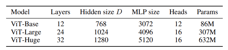
Let’s initialize our model with the above hyperparameters and check the number of parameters with the original PyTorch implementation.
Starting with the Vision Transformer Base hyperparameters which are the default values in the main block. We just need to execute the model.py file.
python model.py
We get the following output.
ViT(
  (patches): CreatePatches(
    (patch): Conv2d(3, 768, kernel_size=(16, 16), stride=(16, 16))
  )
  (attn_layers): ModuleList(
    (0-11): 12 x AttentionBlock(
      (pre_norm): LayerNorm((768,), eps=1e-06, elementwise_affine=True)
      (attention): MultiheadAttention(
        (out_proj): NonDynamicallyQuantizableLinear(in_features=768, out_features=768, bias=True)
      )
      (norm): LayerNorm((768,), eps=1e-06, elementwise_affine=True)
      (MLP): Sequential(
        (0): Linear(in_features=768, out_features=3072, bias=True)
        (1): GELU(approximate='none')
        (2): Dropout(p=0.0, inplace=False)
        (3): Linear(in_features=3072, out_features=768, bias=True)
        (4): Dropout(p=0.0, inplace=False)
      )
    )
  )
  (dropout): Dropout(p=0.0, inplace=False)
  (ln): LayerNorm((768,), eps=1e-06, elementwise_affine=True)
  (head): Linear(in_features=768, out_features=1000, bias=True)
)
86,567,656 total parameters.
86,567,656 training parameters.
Output shape from model: torch.Size([1, 1000])
The above parameters match the PyTorch VIT_B_16 exactly.
Now, changing the hyperparameters for the large model and executing the script again gives the following outputs.
ViT(
  (patches): CreatePatches(
    (patch): Conv2d(3, 1024, kernel_size=(16, 16), stride=(16, 16))
  )
  (attn_layers): ModuleList(
    (0-23): 24 x AttentionBlock(
      (pre_norm): LayerNorm((1024,), eps=1e-06, elementwise_affine=True)
      (attention): MultiheadAttention(
        (out_proj): NonDynamicallyQuantizableLinear(in_features=1024, out_features=1024, bias=True)
      )
      (norm): LayerNorm((1024,), eps=1e-06, elementwise_affine=True)
      (MLP): Sequential(
        (0): Linear(in_features=1024, out_features=4096, bias=True)
        (1): GELU(approximate='none')
        (2): Dropout(p=0.0, inplace=False)
        (3): Linear(in_features=4096, out_features=1024, bias=True)
        (4): Dropout(p=0.0, inplace=False)
      )
    )
  )
  (dropout): Dropout(p=0.0, inplace=False)
  (ln): LayerNorm((1024,), eps=1e-06, elementwise_affine=True)
  (head): Linear(in_features=1024, out_features=1000, bias=True)
)
304,326,632 total parameters.
304,326,632 training parameters.
Output shape from model: torch.Size([1, 1000])
This again matches the VIT_L_16 parameters in Torchvision.
For the huge model though, the PyTorch implementation has a patch size of 14 instead of 16 along with the above hyperparameters from figure 5. So, the model initialization becomes the following.
model = ViT(
        img_size=224,
        patch_size=14,
        embed_dim=1280,
        hidden_dim=5120,
        num_heads=16,
        num_layers=32
    )
Executing the script with the above hyperparameters gives the following output.
ViT(
  (patches): CreatePatches(
    (patch): Conv2d(3, 1280, kernel_size=(14, 14), stride=(14, 14))
  )
  (attn_layers): ModuleList(
    (0-31): 32 x AttentionBlock(
      (pre_norm): LayerNorm((1280,), eps=1e-06, elementwise_affine=True)
      (attention): MultiheadAttention(
        (out_proj): NonDynamicallyQuantizableLinear(in_features=1280, out_features=1280, bias=True)
      )
      (norm): LayerNorm((1280,), eps=1e-06, elementwise_affine=True)
      (MLP): Sequential(
        (0): Linear(in_features=1280, out_features=5120, bias=True)
        (1): GELU(approximate='none')
        (2): Dropout(p=0.0, inplace=False)
        (3): Linear(in_features=5120, out_features=1280, bias=True)
        (4): Dropout(p=0.0, inplace=False)
      )
    )
  )
  (dropout): Dropout(p=0.0, inplace=False)
  (ln): LayerNorm((1280,), eps=1e-06, elementwise_affine=True)
  (head): Linear(in_features=1280, out_features=1000, bias=True)
)
632,045,800 total parameters.
632,045,800 training parameters.
Output shape from model: torch.Size([1, 1000])
The above parameters match the VIT_H_14 SWAG_LINEAR_V1 model from Torchvision.
It looks like our implementation of Vision Transformer from scratch is correct.
Summary and Conclusion
In this article, we implemented the Vision Transformer model from scratch. Along the way, we discussed what each parameter does and why we need certain components in the model. In the next article, we will train the Vision Transformer model from scratch and try to get the best results possible. I hope that this article was worth your time.
If you have any doubts, thoughts, or suggestions, please leave them in the comment section. I will surely address them.
You can contact me using the Contact section. You can also find me on LinkedIn, and X.
References

23 thoughts on “Vision Transformer from Scratch – PyTorch Implementation”