RT-DETR: Paper Explanation and Inference

Detection Transformers have come a long way in computer vision. Starting from the very first DETR paper to RT-DETR, the approach to anchor free real time object detection using Vision Transformers has changed significantly. Focusing on that, in this article, we will discuss the RT-DETR model. Along with that, we will go through the most important sections of the RT-DETR paper.

The RT-DETR (Real Time Detection Transformers) model was introduced by researchers from Baidu in the paper named DETRs Beat YOLOs on Real-time Object Detection. Although the main aim was to create an object detector that is faster and more accurate than YOLO models, the paper covers much more. We will cover that and inference using pretrained RT-DETR models as well in this article.

We will cover the following topics about RT-DETR

• First, we will cover an introduction to RT-DETR while mentioning the issues with current object detectors and the main contributions of the research.
• Second, we will cover the architecture and how it is different from the previous DETR model.
• Third, we will cover the benchmark and performance comparison of RT-DETR with other models.
• Finally, we will run inference using RT-DETR ResNet18, RT-DETR ResNet34, RT-DETR ResNet50, and RT-DETR ResNet101 models.

What are the Issues with Anchor Based Object Detectors?

Anchor based object detection models create several box proposals that we need to filter out during test time. Although automated nowadays, initially anchor selection was mostly manual code, and therefore was a hand-crafted method. One such example is the Faster RCNN model.

Because we have to filter out thousands of boxes during test/inference, this leads to a latency overhead during the forward pass of the model. Removing the dependency on anchor boxes does two things:

• It greatly reduces the complexity of the entire object detection pipeline.
• And it increases forward pass speed as well.

The DERT model was one of the first models to do this. Since then, a lot of research has focused on anchor free Vision Transformer based object detection models.

However, getting Vision Transformer based object detection models to work in real-time with high accuracy is a challenge. On this note, as of writing this, the RT-DETR model is perhaps the best model which is:

• Anchor free
• Faster than most anchor based and CNN based object detectors
• And even more accurate than the previous anchor free, Transformer based and CNN based object detectors

This brings us to the main contributions of the RT-DETR paper:

• It is completely end-to-end and outperforms current object detection models in speed and accuracy.
• Due to the removal of NMS, the inference speed remains stable throughout.
• The paper provides a detailed report on the effect of NMS in object detection.
• RT-DETR provides a methodology for using different decoder layers to adjust inference speed without the need for retraining.

The RT-DETR Architecture

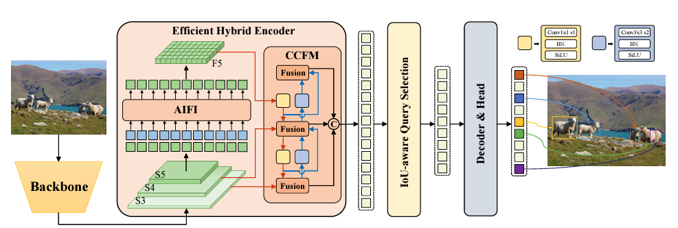
The RT-DETR model consists of three main components:

• Backbone
• Hybrid Encoder
• And a Transformer decoder

The RT-DETR Backbone

In the initial research, the authors experiment with two backbone families, ResNet, and HGNetv2 models.

Instead of selecting just the final feature map from the backbone, the authors choose features from three different levels of the backbone. The last three stages, \({S_3, S_4, S_5}\) go as input to the encoder of RT-DETR.

So, the backbone works as the feature extractor whose feature maps from three scales go to the hybrid encoder.

The RT-DETR Hybrid Encoder

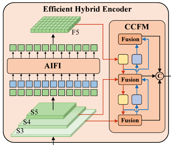
As we discussed previously, the outputs from the last three stages of the backbone are passed as input to the Hybrid Encoder of the model.

The Hybrid Encoder transforms the features into a sequence of image features. For this, it employs two other modules. They are:

• AIFI (Attention based Intra Scale Feature Interaction)
• CCFM (CNN based Cross-scale Feature-fusion Module)

The AIFI module works on the \(S_5\) feature map only to capture a richer semantic concept. This also reduces the complexity and increases the overall accuracy of the model.

On the other hand, CCFM captures the semantic concepts from features \(S_4\) and \(S_5\). The CCFM module contains a Fusion block as well.

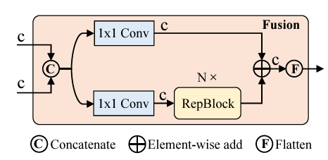
Its role is to fuse features from two adjacent blocks into a new feature which passes through 1×1 convolutions, as we can see in the above image.

The RT-DETR IoU Aware Query Selection and Transformer Decoder

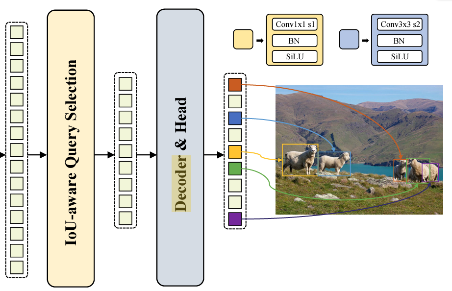
All the image features from the Hybrid Encoder do not go as input to the decoder. Rather, the IoU Aware Query Selection module selects a set of image features as an initial input to the Transformer Decoder.

The Decoder, which consists of auxiliary prediction heads, generates the boxes and the confidence scores.

This covers a very high level overview of the RT-DETR model architecture. In a future post, we will dive deep into the code of the RT-DETR model to understand it further.

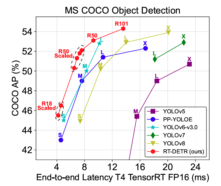
RT-DETR Performance Comparison with Other Models

The RT-DETR model seems to surpass almost all of the previous real-time and end-to-end detectors in terms of speed and the mAP metric. All of this while being smaller (in parameters) than other models.

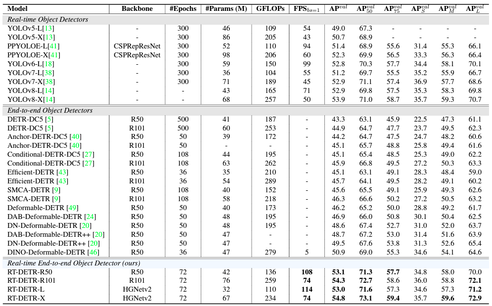
However, it is worth noting that all of the performance comparisons happen on the T4 GPU with TensorRT FP16. It would be interesting to see the performance comparison between the recent YOLO models, and RT-DETR on consumer GPUs (gaming or RTX A series).

Inference using DETR

We have covered a good overview of the RT-DETR model till now. Now, let’s jump to en even interesting part, running inference on images and videos.

Although the authors provide an official repository with PaddlePaddle and PyTorch implementation, it is difficult to run PyTorch inference with that.

For this reason, I have implemented, the pretrained model and code into my vision_transformers library for ResNet-based RTDETR models. We will use this to import the models and run inference on images and videos.

Before that, let’s setup an environment with the major dependencies.

Setting Up the vision_transformers Library

It is recommended to use Anaconda to create and manage the environment for this. The library uses the PyTorch framework. So, we need to install that first with CUDA support.

conda install pytorch torchvision torchaudio pytorch-cuda=11.8 -c pytorch -c nvidia

The next step is cloning the vision_transformers library and installing it. You can do it in any directory of your choice.

git clone https://github.com/sovit-123/vision_transformers.git

Next, enter the directory and install the library.

cd vision_transformers

pip install .

There are other smaller dependencies like OpenCV which you can install as you see fit while running the code.

This completes the entire setup. Now, we can import the library anywhere to run inference using the RT-DETR model.

The Project Directory Structure

The following block shows the entire directory structure where we run the inference.

├── input
├── outputs
├── image_inference.py
├── utils.py
└── video_inference.py

• The input and outputs directories contain the input data and output from the models respectively.
• image_inference.py and video_inference.py scripts are for running inference on images and videos respectively.
• And the utils.py file contains the helper scripts.

This is all the setup we need. Now, we can move to the coding part.

Download Code

Utility Scripts

Let’s start with some utility scripts that we have in the utils.py file.

First is importing the necessary packages, defining the COCO dataset class names and mapping, and the color mapping for bounding box annotations.

import numpy as np
import cv2 
import torch

np.random.seed(42)

mscoco_category2name = {
    1: 'person',
    2: 'bicycle',
    3: 'car',
    4: 'motorcycle',
    5: 'airplane',
    6: 'bus',
    7: 'train',
    8: 'truck',
    9: 'boat',
    10: 'traffic light',
    11: 'fire hydrant',
    13: 'stop sign',
    14: 'parking meter',
    15: 'bench',
    16: 'bird',
    17: 'cat',
    18: 'dog',
    19: 'horse',
    20: 'sheep',
    21: 'cow',
    22: 'elephant',
    23: 'bear',
    24: 'zebra',
    25: 'giraffe',
    27: 'backpack',
    28: 'umbrella',
    31: 'handbag',
    32: 'tie',
    33: 'suitcase',
    34: 'frisbee',
    35: 'skis',
    36: 'snowboard',
    37: 'sports ball',
    38: 'kite',
    39: 'baseball bat',
    40: 'baseball glove',
    41: 'skateboard',
    42: 'surfboard',
    43: 'tennis racket',
    44: 'bottle',
    46: 'wine glass',
    47: 'cup',
    48: 'fork',
    49: 'knife',
    50: 'spoon',
    51: 'bowl',
    52: 'banana',
    53: 'apple',
    54: 'sandwich',
    55: 'orange',
    56: 'broccoli',
    57: 'carrot',
    58: 'hot dog',
    59: 'pizza',
    60: 'donut',
    61: 'cake',
    62: 'chair',
    63: 'couch',
    64: 'potted plant',
    65: 'bed',
    67: 'dining table',
    70: 'toilet',
    72: 'tv',
    73: 'laptop',
    74: 'mouse',
    75: 'remote',
    76: 'keyboard',
    77: 'cell phone',
    78: 'microwave',
    79: 'oven',
    80: 'toaster',
    81: 'sink',
    82: 'refrigerator',
    84: 'book',
    85: 'clock',
    86: 'vase',
    87: 'scissors',
    88: 'teddy bear',
    89: 'hair drier',
    90: 'toothbrush'
}

mscoco_category2label = {k: i for i, k in enumerate(mscoco_category2name.keys())}
mscoco_label2category = {v: k for k, v in mscoco_category2label.items()}

COLORS = np.random.uniform(0, 255, size=(len(mscoco_category2name), 3)) 

We will use the mscoco_label2category dictionary to map the index number from the model output to the class label.

Next, for both image and video inference, we can write a common function to annotate the frames/images with the bounding boxes and class names. The following draw_boxes function does that.

def draw_boxes(outputs, orig_image):
    for i in range(len(outputs['pred_boxes'][0])):
        logits = outputs['pred_logits'][0][i]
        soft_logits = torch.softmax(logits, dim=-1)
        max_index = torch.argmax(soft_logits).cpu()
        class_name = mscoco_category2name[mscoco_label2category[int(max_index.numpy())]]
        
        if soft_logits[max_index] > 0.50:
            box = outputs['pred_boxes'][0][i].cpu().numpy()
            cx, cy, w, h = box
            cx = cx * orig_image.shape[1]
            cy = cy * orig_image.shape[0]
            w = w * orig_image.shape[1]
            h = h * orig_image.shape[0]
            
            x1 = int(cx - (w//2))
            y1 = int(cy - (h//2))
            x2 = int(x1 + w)
            y2 = int(y1 + h)

            color = COLORS[max_index]
            
            cv2.rectangle(
                orig_image,
                (x1, y1),
                (x2, y2),
                thickness=2,
                color=color,
                lineType=cv2.LINE_AA
            )
            
            cv2.putText(
                orig_image,
                text=class_name,
                org=(x1, y1-10),
                fontFace=cv2.FONT_HERSHEY_SIMPLEX,
                fontScale=0.6,
                thickness=2,
                color=color,
                lineType=cv2.LINE_AA
            )
    
    return orig_image

There are a few details that we need to observe in the above code block. The RT-DETR models output a dictionary containing pred_logits and pred_boxes keys.

pred_logits has a shape of [1, 300, 80]. This means the model outputs 300 object queries for an entire image. Furthermore, each query contains the logits for all 80 classes from the COCO dataset. We need to apply Softmax to the logits to get the probability scores and extract the index with the highest score. That index maps to the class name from the above-defined mscoco_label2category.

Coming to the bounding boxes, the model outputs pred_boxes of shape [1, 300, 4]. So, these are 4 coordinates for each of the 300 object queries. These coordinates are in the normalized x center, y center, width, and height format. Just like the YOLO models.

In the above code, we convert them to absolute coordinates and obtain the top-left and bottom-right coordinates after that.

Finally, we annotate the bounding boxes and class names on top of each object that has a probability score of greater than 50%.

Image Inference using RT-DETR

Moving on to image inference using the RT-DETR model. All the code for this resides in the image_inference.py script.

Starting with the imports, defining the argument parser, and the computation device.

from vision_transformers.detection.rtdetr import load_model
from torchvision import transforms
from utils import draw_boxes

import cv2
import torch
import argparse
import os

parser = argparse.ArgumentParser()
parser.add_argument(
    '--model',
    help='model name',
    default='rtdetr_resnet50'
)
parser.add_argument(
    '--input',
    default='input/image_1.jpg'
)
parser.add_argument(
    '--device',
    help='cpu or cuda',
    default=torch.device('cuda:0' if torch.cuda.is_available() else 'cpu')
)
args = parser.parse_args()

OUT_DIR = os.path.join('outputs')
os.makedirs(OUT_DIR, exist_ok=True)

device = args.device

We import the load_model function to initialize the RT-DETR model from the vision_transformers library. Along with that, we also import draw_boxes from utils.

The argument parser defines three command line arguments: one for the model name, one for the input image, and one for the computation device.

We can choose between 4 different models and by default it is the one with a ResNet50 backbone.

# Load model.
# Choose model between,
# rtdetr_resnet18, rtdetr_resnet34, rtdetr_resnet50, rtdetr_resnet101
model = load_model(args.model)
model.eval().to(device)

# Total parameters and trainable parameters.
total_params = sum(p.numel() for p in model.parameters())
print(f"{total_params:,} total parameters.")
total_trainable_params = sum(
    p.numel() for p in model.parameters() if p.requires_grad)
print(f"{total_trainable_params:,} training parameters.")

Next, let’s load the image, apply the transforms, and carry out the forward pass.

image = cv2.imread(args.input)
orig_image = image.copy()
image = cv2.cvtColor(image, cv2.COLOR_BGR2RGB)
image = cv2.resize(image, (640, 640))

transform = transforms.Compose([
    transforms.ToPILImage(),
    transforms.ToTensor(),
    transforms.ConvertImageDtype(torch.float),
])

image = transform(image)
image = image.unsqueeze(0).to(device)

# Forward pass.
with torch.no_grad():
    outputs = model(image)

orig_image = draw_boxes(outputs, orig_image)

cv2.imshow('Image', orig_image)
cv2.waitKey(0)

file_name =  args.input.split(os.path.sep)[-1]
cv2.imwrite(os.path.join(OUT_DIR, file_name), orig_image)

The models were trained on 640×640 images and that is the resolution we are resizing all the images to here. After the forward pass, we call the draw_boxes function, visualize the output on the screen, and save the result in the outputs directory.

We can execute the following command in the terminal to run the inference.

python image_inference.py

Following is the output for this.

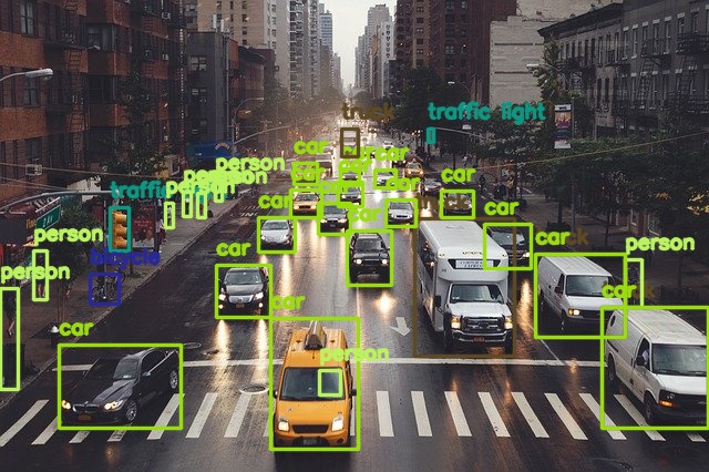
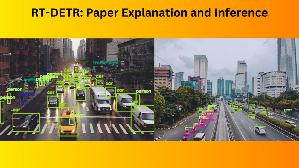
The RT-DETR ResNet50 model can detect almost all the objects in the image. Even the person inside the car and the far away traffic light are detected. This is impressive.

Now, let’s consider a slightly more challenging scene with more far away traffic and vehicles.

python image_inference.py --input input/image_3.jpg --model rtdetr_resnet101

This time we employ the RT-DETR ResNet101 model and get the following result.

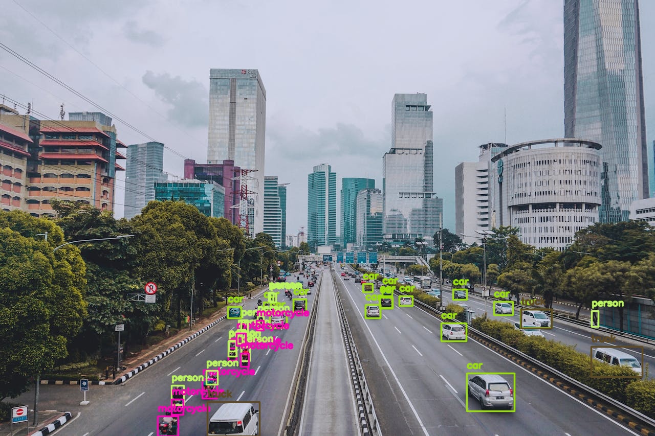
Although the model is confusing between a car and a truck for one of the objects, overall it is doing very well. It can detect the persons on top of the motorcycles, even the ones which are far away.

Video Inference using RT-DETR

Video inference will remain just as simple. A lot of the code will remain the same and we just need to loop over the video frames. The code for this goes into the video_inference.py file.

from vision_transformers.detection.rtdetr import load_model
from torchvision import transforms
from utils import draw_boxes

import cv2
import torch
import argparse
import os
import time

parser = argparse.ArgumentParser()
parser.add_argument(
    '--model',
    help='model name',
    default='rtdetr_resnet50'
)
parser.add_argument(
    '--input',
    default='input/video_1.mp4'
)
parser.add_argument(
    '--device',
    help='cpu or cuda',
    default=torch.device('cuda:0' if torch.cuda.is_available() else 'cpu')
)
args = parser.parse_args()

OUT_DIR = os.path.join('outputs')
os.makedirs(OUT_DIR, exist_ok=True)

device = args.device

# Load model.
# Choose model between,
# rtdetr_resnet18, rtdetr_resnet34, rtdetr_resnet50, rtdetr_resnet101
model = load_model(args.model)
model.eval().to(device)

# Total parameters and trainable parameters.
total_params = sum(p.numel() for p in model.parameters())
print(f"{total_params:,} total parameters.")
total_trainable_params = sum(
    p.numel() for p in model.parameters() if p.requires_grad)
print(f"{total_trainable_params:,} training parameters.")

The code till the loading of the model remains the same.

Next is loading the video, defining the VideoWriter object, looping over the frames, and carrying out inference.

# Load video and read data.
cap = cv2.VideoCapture(args.input)
frame_width = int(cap.get(3))
frame_height = int(cap.get(4))
vid_fps = int(cap.get(5))
file_name = args.input.split(os.path.sep)[-1].split('.')[0]
out = cv2.VideoWriter(
    f"{OUT_DIR}/{file_name}.mp4", 
    cv2.VideoWriter_fourcc(*'mp4v'), vid_fps, 
    (frame_width, frame_height)
)

# Inference transforms.
transform = transforms.Compose([
    transforms.ToPILImage(),
    transforms.Resize((640, 640)),
    transforms.ToTensor(),
    transforms.ConvertImageDtype(torch.float)
])

frame_count = 0
total_fps = 0
while cap.isOpened():
    ret, frame = cap.read()
    if ret:
        frame_count += 1
        image = cv2.cvtColor(frame, cv2.COLOR_BGR2RGB)
        image = transform(image).unsqueeze(0).to(device)

        start_time = time.time()
        with torch.no_grad():
            outputs = model(image)
        end_time = time.time()
        fps = 1 / (end_time - start_time)
        total_fps += fps

        frame = draw_boxes(outputs, frame)
        
        cv2.putText(
            frame,
            text=f"FPS: {fps:.1f}",
            org=(15, 25),
            fontFace=cv2.FONT_HERSHEY_SIMPLEX,
            fontScale=1.0,
            thickness=2,
            color=(0, 255, 0),
            lineType=cv2.LINE_AA
        )
        out.write(frame)
        cv2.imshow('Image', frame)
        if cv2.waitKey(1) & 0xFF == ord('q'):
            break

    else:
        break

# Release VideoCapture().
cap.release()
# Close all frames and video windows.
cv2.destroyAllWindows()

# Calculate and print the average FPS.
avg_fps = total_fps / frame_count
print(f"Average FPS: {avg_fps:.3f}")

Rest of the code like transforms and annotations remains the same. Additionally, we annotate the FPS on top of each frame.

Let’s take a look at a result using the RT-DETR ResNet50 model.

python video_inference.py --input input/video_2.mp4 --model rtdetr_resnet50

Following is the result.

On an RTX 3080 GPU, the model runs at 46 FPS on average. The detections are quite good as well.

Now let’s draw a comparison between all 4 models on the same video.

As expected the model with the ResNet18 backbone runs the fastest and the one with ResNet101 captures smaller objects better. RT-DETR ResNet34 model seems like a good tradeoff between speed and accuracy.

Summary and Conclusion

In this article, we covered the RT-DETR model. We went through the model architecture overview and carried out inference on images and videos. This gave us an overall idea of the model’s performance. In future posts, we will try to dive deeper into the coding aspects of the RT-DETR model. I hope this article was worth your time.

If you have any doubts, thoughts, or suggestions, please leave them in the comment section. I will surely address them.

You can contact me using the Contact section. You can also find me on LinkedIn, and Twitter.

References

• DETRs Beat YOLOs on Real-time Object Detection