Training Vision Transformer from Scratch

In the previous article, we implemented the Vision Transformer model from scratch. We also verified our implementation against the Torchvision implementation and found them exactly the same. In this article, we will take it a step further. We will be training the same Vision Transformer model from scratch on two medium-scale datasets.

figure 1. some output gifs here…

Training Vision Transformer models, or as a matter of fact any transformer model is a challenging task. They often require huge datasets to reach an acceptable accuracy. However, just like CNNs, we can make smart hyperparameter choices while training transformer based models. These choices, although not state-of-the-art, will give us excellent results even on medium-scale datasets.

Here are the topics that we will cover in this article

• We will start with a discussion of the datasets that we will train the Vision Transformer model on.
  • We will train on two datasets, one medical imaging dataset, and the classic CIFAR10 dataset.
• Next, we will discuss how the project is structured and what are the important files to focus on.
• Then we will move on to the dataset preparation and augmentation techniques for the same.
• We will follow this with training.
• Finally, we will run inference on some unseen images from the internet.

Datasets for Training the Vision Transformer Model from Scratch

We will run training experiments on two datasets:

• The CIFAR10 dataset
• A brain tumor MRI dataset

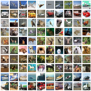
The CIFAR10 Dataset

The CIFAR10 is one of the most famous benchmarking datasets in the field of computer vision. Whenever creating a model from scratch, almost always there would be at least one training experiment on the CIFAR10 dataset. This is because it is not that easy to get state-of-the-art accuracy on the CIFAR10 dataset when training from scratch.

It contains 10 classes across 60000 images amounting to 6000 images per class. The classes are:

• airplane
• automobile
• bird
• cat
• deer
• dog
• frog
• horse
• ship
• truck

Furthermore, all the images are 32×32 RGB images. The small resolution of the images is what makes the dataset even more challenging.

The CIFAR10 dataset is already part of the Torchvision datasets where 50000 images are for training and 10000 are for validation. We will directly load the dataset and need not download it separately.

As the original Vision Transformer paper does not report the CIFAR10 training results from scratch, we will have to make our own hyperparameter choices.

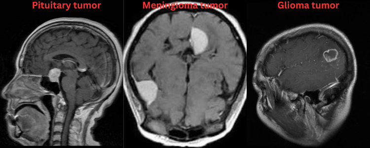
The Brain MRI Dataset

The second dataset that we will use for training is the Brain Tumor MRI dataset from Kaggle.

This dataset contains images belonging to 4 classes:

• Glioma brain tumor MRI images
• Meningioma brain tumor MRI images
• Pituitary brain tumor MRI images
• Normal brain MRI images

However, we will use only the images containing brain tumors for training. So, only three classes will be used. This amounts to 6307 glioma, 6391 meningioma, and 5908 pituitary tumor images.

The authors of the dataset have already applied augmentation to the images. These augmentations include:

• Salt and Pepper Noise
• Histogram Equalization
• Rotation
• Brightness Adjustment
• Horizontal and Vertical Flipping

For this reason, we will not add any augmentation during training.

Downloading and extracting the dataset will give the following directory structure.

Data/
├── Normal [3066 entries exceeds filelimit, not opening dir]
└── Tumor
    ├── glioma_tumor
    ├── meningioma_tumor
    └── pituitary_tumor

The dataset extracts into the Data directory. There are 3066 images belonging to the Normal class. However, we will only use the data present in the Tumor directory where each image is present inside their class directory.

If you plan on executing the training yourself, go ahead and download the dataset.

The Entire Project Directory Structure

Here is the entire directory structure.

├── input
│   ├── data
│   ├── Data
│   └── inference_data
├── outputs
│   ├── cifar10
│   ├── inference_results
│   └── tumor
└── src
    ├── class_names.py
    ├── datasets.py
    ├── inference.py
    ├── model.py
    ├── train_cifar10.py
    ├── train.py
    └── utils.py

• The input directory contains the CIFAR10 dataset inside the data directory and the brain MRI images inside the Data directory. The CIFAR10 dataset will be automatically downloaded the first time we execute the training script for the same. It also contains an inference_data directory with two subdirectories for each of the datasets. These are images from the internet that we will run inference on after the training experiment.
• The outputs directory contains the training experiment results and also the results from the inference.
• In the src directory, we have several Python files. We will go through the necessary ones in their own subsections.

The trained models and the Python files are provided via the download section. In case you want to run the training experiment, please download the brain MRI dataset.

PyTorch Version

The code in this article has been developed using PyTorch 2.0.1. However, PyTorch >= 1.13.0 should work without any issues.

Training Vision Transformer from Scratch using PyTorch

As you may see in the above directory structure, there are two training scripts, train.py and train_cifar10.py. We will carry out two training experiments, one for the tumor dataset, and another for the CIFAR10 dataset. This will allow us to know how to tune different hyperparameters and how to scale the model when dealing with different datasets.

The CIFAR10 training script does not rely on the datasets.py file for the dataset preparation as we can load the dataset directory from the torchvision module. It does rely on the other helper and utility scripts though. The train.py contains its dataset preparation code in datasets.py.

First, we will discuss the training procedure for the brain tumor MRI images and then move on to the CIFAR10 training.

We will not go through the Vision Transformer model preparation code in this article as we already did that in detail in the previous one. If you want a detailed explanation, you may go through implementing Vision Transformer from scratch before moving ahead.

Download Code

Training Vision Transformer on Brain Tumor MRI Images

Let’s start with the utility and helper scripts in the utils.py file. It contains a class to save the best model according to the lowest loss, a function to save the model after each epoch, and also a function to save the accuracy and loss graphs.

The Utility Scripts

The following code resides in the utils.py file and is common for both, the brain tumor MRI training and the CIFAR10 training.

import torch
import matplotlib
import matplotlib.pyplot as plt
import os

matplotlib.style.use('ggplot')

class SaveBestModel:
    """
    Class to save the best model while training. If the current epoch's 
    validation loss is less than the previous least less, then save the
    model state.
    """
    def __init__(
        self, best_valid_loss=float('inf')
    ):
        self.best_valid_loss = best_valid_loss
        
    def __call__(
        self, current_valid_loss, epoch, model, out_dir
    ):
        if current_valid_loss < self.best_valid_loss:
            self.best_valid_loss = current_valid_loss
            print(f"\nBest validation loss: {self.best_valid_loss}")
            print(f"\nSaving best model for epoch: {epoch+1}\n")
            torch.save({
                'epoch': epoch+1,
                'model_state_dict': model.state_dict(),
                }, os.path.join(out_dir, 'best_model.pth'))

def save_model(epochs, model, optimizer, criterion, out_dir, name):
    """
    Function to save the trained model to disk.
    """
    torch.save({
                'epoch': epochs,
                'model_state_dict': model.state_dict(),
                'optimizer_state_dict': optimizer.state_dict(),
                'loss': criterion,
                }, os.path.join(out_dir, name+'.pth'))

def save_plots(train_acc, valid_acc, train_loss, valid_loss, out_dir):
    """
    Function to save the loss and accuracy plots to disk.
    """
    # Accuracy plots.
    plt.figure(figsize=(10, 7))
    plt.plot(
        train_acc, color='tab:blue', linestyle='-', 
        label='train accuracy'
    )
    plt.plot(
        valid_acc, color='tab:red', linestyle='-', 
        label='validataion accuracy'
    )
    plt.xlabel('Epochs')
    plt.ylabel('Accuracy')
    plt.legend()
    plt.savefig(os.path.join(out_dir, 'accuracy.png'))
    
    # Loss plots.
    plt.figure(figsize=(10, 7))
    plt.plot(
        train_loss, color='tab:blue', linestyle='-', 
        label='train loss'
    )
    plt.plot(
        valid_loss, color='tab:red', linestyle='-', 
        label='validataion loss'
    )
    plt.xlabel('Epochs')
    plt.ylabel('Loss')
    plt.legend()
    plt.savefig(os.path.join(out_dir, 'loss.png')) 

An object of the SaveBestModel class saves the model weights to the disk whenever the current validation loss is lower than the previous one. The save_model() function saves the model weights along with the optimizer state after every epoch. This is helpful for resuming training in case we want it. And the save_plots() function saves the accuracy and loss plots.

The Dataset Preparation

The code in the datasets.py creates the datasets and data loaders for the brain tumor MRI dataset training. We need to create custom dataset functions for this.

Let’s start with the imports and define some constants.

import os
import torch

from torchvision import datasets, transforms
from torch.utils.data import DataLoader, Subset

# Required constants.
ROOT_DIR = os.path.join(
    '..', 'input', 'Data', 'Tumor'
)
IMAGE_SIZE = 224 # Image size of resize when applying transforms.
NUM_WORKERS = 4 # Number of parallel processes for data preparation.
VALID_SPLIT = 0.15 # Ratio of data for validation

We define the ROOT_DIR as the path to the directory containing the subdirectories for each of the tumor classes. As discussed earlier, we will only train on the tumor images and leave the normal brain MRI images.

Then, we define the image size for training which is 224×224, the number of parallel workers as 4, and the validation split as 15%. This amounts to 15816 training images and 2790 validation images. We need to be careful to include the majority of the images in the training set when training the Vision Transformer model from scratch. Otherwise, it may get to learn properly when dealing with such difficult datasets.

Coming to the training and validation transforms.

# Training transforms.
def get_train_transform(image_size):
    train_transform = transforms.Compose([
        transforms.Resize((image_size, image_size)),
        transforms.CenterCrop(224),
        # transforms.RandomHorizontalFlip(p=0.5),
        # transforms.RandomVerticalFlip(p=0.5),
        # transforms.RandomRotation(35),
        transforms.ToTensor(),
        transforms.Normalize(
            mean=[0.5, 0.5, 0.5],
            std=[0.5, 0.5, 0.5]
        )
    ])
    return train_transform

# Validation transforms.
def get_valid_transform(image_size):
    valid_transform = transforms.Compose([
        transforms.Resize((image_size, image_size)),
        transforms.CenterCrop(224),
        transforms.ToTensor(),
        transforms.Normalize(
            mean=[0.5, 0.5, 0.5],
            std=[0.5, 0.5, 0.5]
        )
    ])
    return valid_transform

The above two functions contain the transforms. As you may see, we do not apply augmentations to the training set as the images are already augmented. However, they are commented out in case we want to experiment with more datasets in the future. For both sets, we resize the images, crop to the same size (effectively, no cropping), convert the images to tensors, and normalize them.

Next, we need to define the functions for creating the datasets and data loaders.

def get_datasets():
    """
    Function to prepare the Datasets.
    Returns the training and validation datasets along 
    with the class names.
    """
    dataset = datasets.ImageFolder(
        ROOT_DIR, 
        transform=(get_train_transform(IMAGE_SIZE))
    )
    dataset_test = datasets.ImageFolder(
        ROOT_DIR, 
        transform=(get_valid_transform(IMAGE_SIZE))
    )
    dataset_size = len(dataset)

    # Calculate the validation dataset size.
    valid_size = int(VALID_SPLIT*dataset_size)
    # Radomize the data indices.
    indices = torch.randperm(len(dataset)).tolist()
    # Training and validation sets.
    dataset_train = Subset(dataset, indices[:-valid_size])
    dataset_valid = Subset(dataset_test, indices[-valid_size:])

    return dataset_train, dataset_valid, dataset.classes

def get_data_loaders(dataset_train, dataset_valid, batch_size):
    """
    Prepares the training and validation data loaders.
    :param dataset_train: The training dataset.
    :param dataset_valid: The validation dataset.
    Returns the training and validation data loaders.
    """
    train_loader = DataLoader(
        dataset_train, batch_size=batch_size, 
        shuffle=True, num_workers=NUM_WORKERS
    )
    valid_loader = DataLoader(
        dataset_valid, batch_size=batch_size, 
        shuffle=False, num_workers=NUM_WORKERS
    )
    return train_loader, valid_loader 

We have all the images in their respective class directories without any split. So, we create two similar datasets, dataset and dataset_test. Then we calculate the validation size (line 59), create random indices (line 61), and create dataset_train and dataset_valid subsets from the dataset and dataset_test respectively (lines 63 and 64). This works very well when not having splits by default.

The get_data_loaders() function simply returns the training and validation data loaders using the respective datasets.

The Brain Tumor MRI Dataset Training Script

The train.py script contains all the code to start training on the brain tumor MRI dataset. Let’s discuss the code first.

The following block contains all the import statements and the argument parsers.

import torch
import argparse
import torch.nn as nn
import torch.optim as optim
import os

from tqdm.auto import tqdm
from model import ViT
from datasets import get_datasets, get_data_loaders
from utils import save_model, save_plots, SaveBestModel

seed = 42
torch.manual_seed(seed)
torch.cuda.manual_seed(seed)
torch.backends.cudnn.deterministic = True
torch.backends.cudnn.benchmark = True

# Construct the argument parser.
parser = argparse.ArgumentParser()
parser.add_argument(
    '-e', '--epochs',
    type=int,
    default=10,
    help='Number of epochs to train our network for'
)
parser.add_argument(
    '-lr', '--learning-rate',
    type=float,
    dest='learning_rate',
    default=0.001,
    help='Learning rate for training the model'
)
parser.add_argument(
    '-b', '--batch-size',
    dest='batch_size',
    default=32,
    type=int
)
parser.add_argument(
    '-ft', '--fine-tune',
    dest='fine_tune' ,
    action='store_true',
    help='pass this to fine tune all layers'
)
parser.add_argument(
    '--save-name',
    dest='save_name',
    default='model',
    help='file name of the final model to save'
)
# Model args.
parser.add_argument(
    '--in-channels',
    dest='in_channels',
    default=3,
    type=int,
    help='image input channels, RGB: 3, Gray: 1'
)
parser.add_argument(
    '--embed-dim',
    dest='embed_dim',
    default=768,
    type=int,
    help='embedding dimension'
)
parser.add_argument(
    '--hidden-dim',
    dest='hidden_dim',
    default=3072,
    type=int,
    help='hidden dimension for linear layers, essentialy embed_dim*4'
)
parser.add_argument(
    '--num-heads',
    dest='num_heads',
    default=12,
    type=int,
    help='number of attention heads'
)
parser.add_argument(
    '--num-layers',
    dest='num_layers',
    default=12,
    type=int,
    help='number of MHSA layers'
)
parser.add_argument(
    '--dropout',
    default=0.0,
    type=float,
    help='global dropout value for model layers'
)
args = parser.parse_args()

First, we import all the necessary modules and libraries, then we set the seed for reproducibility. We have a lot of command line arguments. Along with the common ones like the number of epochs, batch size, and learning rate, we define a lot of model architecture specific ones as well. These include arguments for the embedding dimension, hidden dimension, number of attention heads, and the number of multi-head attention layers among others. These help us control the model size and scale directly when starting the training.

Next, we have the training and validation functions.

# Training function.
def train(model, trainloader, optimizer, criterion):
    model.train()
    print('Training')
    train_running_loss = 0.0
    train_running_correct = 0
    counter = 0
    for i, data in tqdm(enumerate(trainloader), total=len(trainloader)):
        counter += 1
        image, labels = data
        image = image.to(device)
        labels = labels.to(device)
        optimizer.zero_grad()
        # Forward pass.
        outputs = model(image)
        # Calculate the loss.
        loss = criterion(outputs, labels)
        train_running_loss += loss.item()
        # Calculate the accuracy.
        _, preds = torch.max(outputs.data, 1)
        train_running_correct += (preds == labels).sum().item()
        # Backpropagation.
        loss.backward()
        # Update the weights.
        optimizer.step()
    
    # Loss and accuracy for the complete epoch.
    epoch_loss = train_running_loss / counter
    epoch_acc = 100. * (train_running_correct / len(trainloader.dataset))
    return epoch_loss, epoch_acc

# Validation function.
def validate(model, testloader, criterion):
    model.eval()
    print('Validation')
    valid_running_loss = 0.0
    valid_running_correct = 0
    counter = 0

    with torch.no_grad():
        for i, data in tqdm(enumerate(testloader), total=len(testloader)):
            counter += 1
            
            image, labels = data
            image = image.to(device)
            labels = labels.to(device)
            # Forward pass.
            outputs = model(image)
            # Calculate the loss.
            loss = criterion(outputs, labels)
            valid_running_loss += loss.item()
            # Calculate the accuracy.
            _, preds = torch.max(outputs.data, 1)
            valid_running_correct += (preds == labels).sum().item()
        
    # Loss and accuracy for the complete epoch.
    epoch_loss = valid_running_loss / counter
    epoch_acc = 100. * (valid_running_correct / len(testloader.dataset))
    return epoch_loss, epoch_acc

The above are two very generic image classification training and validation functions.

Then we have the main block which is quite large.

if __name__ == '__main__':
    # Create a directory with the model name for outputs.
    out_dir = os.path.join('..', 'outputs', 'tumor')
    os.makedirs(out_dir, exist_ok=True)
    # Load the training and validation datasets.
    dataset_train, dataset_valid, dataset_classes = get_datasets()
    print(f"[INFO]: Number of training images: {len(dataset_train)}")
    print(f"[INFO]: Number of validation images: {len(dataset_valid)}")
    print(f"[INFO]: Classes: {dataset_classes}")
    # Load the training and validation data loaders.
    train_loader, valid_loader = get_data_loaders(
        dataset_train, dataset_valid, batch_size=args.batch_size
    )

    # Learning_parameters.
    lr = args.learning_rate
    epochs = args.epochs
    device = ('cuda' if torch.cuda.is_available() else 'cpu')
    print(f"Computation device: {device}")
    print(f"Learning rate: {lr}")
    print(f"Epochs to train for: {epochs}\n")

    # Load the model.
    model = ViT(
        img_size=224, 
        in_channels=args.in_channels,
        embed_dim=args.embed_dim,
        hidden_dim=args.hidden_dim,
        num_heads=args.num_heads,
        num_layers=args.num_layers,
        dropout=args.dropout,
        num_classes=len(dataset_classes)
    ).to(device)
    print(model)
    
    # Total parameters and trainable parameters.
    total_params = sum(p.numel() for p in model.parameters())
    print(f"{total_params:,} total parameters.")
    total_trainable_params = sum(
        p.numel() for p in model.parameters() if p.requires_grad)
    print(f"{total_trainable_params:,} training parameters.")

    # Optimizer.
    optimizer = optim.AdamW(
        model.parameters(), 
        lr=lr,
        betas=(0.9, 0.95),
        eps=0.00001
    )
    # Loss function.
    criterion = nn.CrossEntropyLoss()

    # Initialize `SaveBestModel` class.
    save_best_model = SaveBestModel()

    # LR scheduler.
    scheduler = optim.lr_scheduler.StepLR(
        optimizer, step_size=10, gamma=0.1, verbose=True
    )

    # Lists to keep track of losses and accuracies.
    train_loss, valid_loss = [], []
    train_acc, valid_acc = [], []
    # Start the training.
    for epoch in range(epochs):
        print(f"[INFO]: Epoch {epoch+1} of {epochs}")
        train_epoch_loss, train_epoch_acc = train(
            model, train_loader, optimizer, criterion
        )
        valid_epoch_loss, valid_epoch_acc = validate(
            model, valid_loader, criterion
        )
        train_loss.append(train_epoch_loss)
        valid_loss.append(valid_epoch_loss)
        train_acc.append(train_epoch_acc)
        valid_acc.append(valid_epoch_acc)
        print(f"Training loss: {train_epoch_loss:.3f}, training acc: {train_epoch_acc:.3f}")
        print(f"Validation loss: {valid_epoch_loss:.3f}, validation acc: {valid_epoch_acc:.3f}")
        save_best_model(valid_epoch_loss, epoch, model, out_dir)
        scheduler.step()
        print('-'*50)

    # Save the trained model weights.
    save_model(epochs, model, optimizer, criterion, out_dir, args.save_name)
    # Save the loss and accuracy plots.
    save_plots(train_acc, valid_acc, train_loss, valid_loss, out_dir)
    print('TRAINING COMPLETE')

The main block carries out the training in the following order:

• We start with the preparation of the datasets and data loaders.
• Then we define the model, the optimizer, and the loss function.
• We also define the learning rate scheduler which reduces the learning rate by a factor of 10 every 10 epochs.
• Finally, we have the training loop and after training, we save the loss & accuracy plots to the disk.

That’s all we need for the training script.

Executing Script to Train Vision Transformer from Scratch on the Brain Tumor MRI Dataset

Note: All training and inference experiments for this post were conducted on a machine with 10 GB RTX 3080 GPU, 10th generation i7 CPU, and 32 GB of RAM.

We can start the training by executing the following command from the terminal within the src directory.

python train.py --learning-rate 0.00005 --epochs 20 --batch-size 32

We train the Vision Transformer model with an initial learning rate of 0.0005, for 20 epochs, with a batch size of 32.

Notice that we do not use any model specific hyperparameters. So, by default, the base Vision Transformer with 85 million parameters gets created.

Here are the truncated outputs from the terminal.

[INFO]: Epoch 1 of 20
Training
100%|████████████████████████████████████████████████████████████████████████████████████████████████████████████████████████████████████████████████████████████████████████████| 495/495 [02:12<00:00,  3.74it/s]
Validation
100%|██████████████████████████████████████████████████████████████████████████████████████████████████████████████████████████████████████████████████████████████████████████████| 88/88 [00:07<00:00, 11.36it/s]
Training loss: 0.786, training acc: 63.847
Validation loss: 0.581, validation acc: 75.520

Best validation loss: 0.5812399753115394

Saving best model for epoch: 1

Adjusting learning rate of group 0 to 5.0000e-05.
--------------------------------------------------
[INFO]: Epoch 2 of 20
Training
100%|████████████████████████████████████████████████████████████████████████████████████████████████████████████████████████████████████████████████████████████████████████████| 495/495 [02:11<00:00,  3.75it/s]
Validation
100%|██████████████████████████████████████████████████████████████████████████████████████████████████████████████████████████████████████████████████████████████████████████████| 88/88 [00:07<00:00, 11.52it/s]
Training loss: 0.543, training acc: 77.238
Validation loss: 0.494, validation acc: 79.391

Best validation loss: 0.49426683817397465

Saving best model for epoch: 2

Adjusting learning rate of group 0 to 5.0000e-05.
--------------------------------------------------
.
.
.
[INFO]: Epoch 11 of 20
Training
100%|████████████████████████████████████████████████████████████████████████████████████████████████████████████████████████████████████████████████████████████████████████████| 495/495 [02:08<00:00,  3.85it/s]
Validation
100%|██████████████████████████████████████████████████████████████████████████████████████████████████████████████████████████████████████████████████████████████████████████████| 88/88 [00:07<00:00, 11.60it/s]
Training loss: 0.026, training acc: 99.071
Validation loss: 0.226, validation acc: 93.943

Best validation loss: 0.22607207803362558

Saving best model for epoch: 11

Adjusting learning rate of group 0 to 5.0000e-06.
--------------------------------------------------
.
.
.
[INFO]: Epoch 20 of 20
Training
100%|████████████████████████████████████████████████████████████████████████████████████████████████████████████████████████████████████████████████████████████████████████████| 495/495 [02:08<00:00,  3.84it/s]
Validation
100%|██████████████████████████████████████████████████████████████████████████████████████████████████████████████████████████████████████████████████████████████████████████████| 88/88 [00:07<00:00, 11.54it/s]
Training loss: 0.003, training acc: 99.867
Validation loss: 0.369, validation acc: 94.014
Adjusting learning rate of group 0 to 5.0000e-07.
--------------------------------------------------
TRAINING COMPLETE

The best model was saved after epoch 11 with a validation loss of 0.22 and a validation accuracy of 93.43%. These are really good numbers when training a Vision Transformer model from scratch.

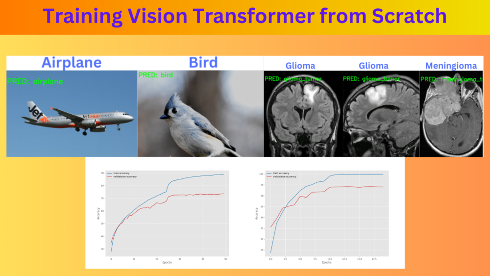
These training results will be present in outputs/tumor directory. Here are the accuracy and loss graphs.

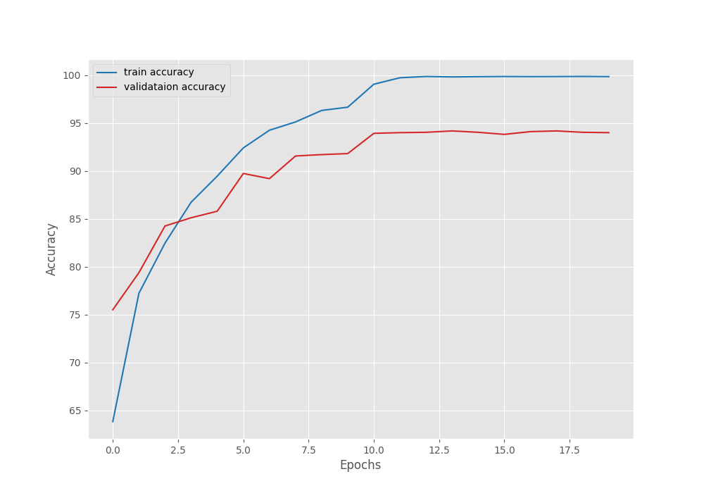
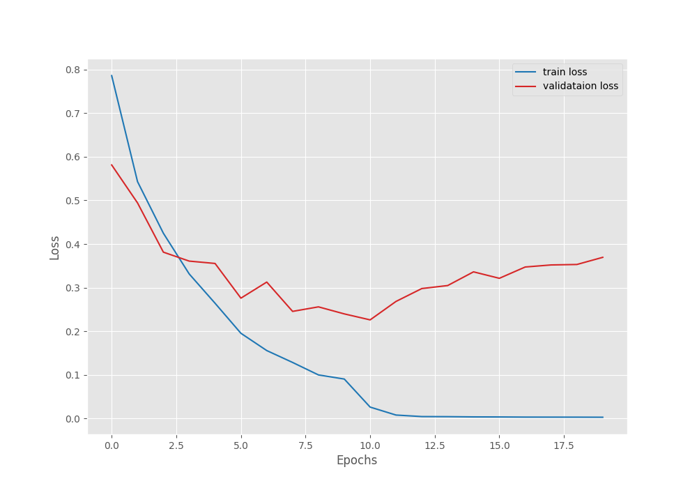
It is clear from the above graphs that the model started to overfit from epoch 12. Maybe a bit more regularization is needed. We can even add more augmentations to the images that are not part of the default dataset preparation stage. For now, we have a good model with us that we can use for inference.

The Inference Script

Let’s move ahead into the inference part using the best model that we trained on the tumor MRI dataset.

The inference code is present in the inference.py file. It can handle inference for both, the MRI dataset trained model and the CIFAR10 trained model. We will go through the CIFAR10 training pipeline after this.

First, we have the import statements, the argument parsers, and a few constants.

import torch
import numpy as np
import cv2
import os
import torch.nn.functional as F
import torchvision.transforms as transforms
import glob
import argparse
import pathlib

from model import ViT

# Construct the argument parser.
parser = argparse.ArgumentParser()
parser.add_argument(
    '-w', '--weights', 
    required=True,
    help='path to the model weights',
)
# Dataset arguments.
parser.add_argument(
    '--num-classes', 
    dest='num_classes',
    default=1000,
    type=int,
    help='number of classes for the pretrained model weights'
)
parser.add_argument(
    '--input',
    required=True,
    help='path to the input directory containing data'
)
parser.add_argument(
    '--data',
    required=True,
    choices=['tumor', 'cifar10'],
    help='name of dataset on which the model was trained'
)
# Model args.
parser.add_argument(
    '--in-channels',
    dest='in_channels',
    default=3,
    type=int,
    help='image input channels, RGB: 3, Gray: 1'
)
parser.add_argument(
    '--embed-dim',
    dest='embed_dim',
    default=768,
    type=int,
    help='embedding dimension'
)
parser.add_argument(
    '--hidden-dim',
    dest='hidden_dim',
    default=3072,
    type=int,
    help='hidden dimension for linear layers, essentialy embed_dim*4'
)
parser.add_argument(
    '--num-heads',
    dest='num_heads',
    default=12,
    type=int,
    help='number of attention heads'
)
parser.add_argument(
    '--num-layers',
    dest='num_layers',
    default=12,
    type=int,
    help='number of MHSA layers'
)
parser.add_argument(
    '--dropout',
    default=0.0,
    type=float,
    help='global dropout value for model layers'
)
args = parser.parse_args()

# Constants and other configurations.
DEVICE = torch.device('cuda:0' if torch.cuda.is_available() else 'cpu')
DEVICE = 'cpu'
IMAGE_RESIZE = 224

In the above code block, there are a few essential command line arguments that we need to know about.

• --num-classes: We can train our model on any dataset and we may need to initialize the model again before loading the weights. So, this argument will help us initialize the last classification layer of the model according to the weights and dataset that the model was trained on.
• --weights: This is simply the path to the trained weights file.
• --data: Right now, there are two choices, tumor and cifar10. According to the argument the class names will be chosen from the class_names.py file. This way it becomes easier to expand to other dataset experimentation as well.
• Following that we have all the model related arguments just like we had in training. This will allow us to correctly create the model so that the weight files do not mismatch.

Next, we have a few helper functions and the validation transforms.

# Validation transforms
def get_test_transform(image_size):
    test_transform = transforms.Compose([
        transforms.ToPILImage(),
        transforms.Resize((image_size, image_size)),
        transforms.CenterCrop(224),
        transforms.ToTensor(),
        transforms.Normalize(
            mean=[0.5, 0.5, 0.5],
            std=[0.5, 0.5, 0.5]
        )
    ])
    return test_transform

def annotate_image(image, output_class):
    pred_name = CLASS_NAMES[int(output_class)]
    print(pred_name)
    # pred_name = str(''.join(pred_name.split('.')[1]))
    cv2.putText(
        image, 
        f"PRED: {pred_name}", 
        (5, 55), 
        cv2.FONT_HERSHEY_SIMPLEX, 
        1, 
        (0, 255, 0), 
        2, 
        lineType=cv2.LINE_AA
    )
    return image

def inference(model, testloader, orig_image, image_name, DEVICE):
    """
    Function to run inference.

    :param model: The trained model.
    :param testloader: The test data loader.
    :param orig_image: The original image.
    :param image_name: The file name.
    :param DEVICE: The computation device.
    """
    model.eval()
    counter = 0
    with torch.no_grad():
        counter += 1
        image = testloader
        image = image.to(DEVICE)

        # Forward pass.
        outputs = model(image)
    # Softmax probabilities.
    predictions = F.softmax(outputs, dim=1).cpu().numpy()
    # Predicted class number.
    output_class = np.argmax(predictions)
    # Show and save the results.
    result = annotate_image(orig_image, output_class)
    return result

We first define the transforms that we will need for inference. These include all the transforms that we had for the validation dataset during training.

For every image result, we will annotate it with the predicted class. The annotate_image() function does that. The inference() function will carry out the forward pass of an image tensor through the model.

Finally, we have the main block.

if __name__ == '__main__':
    if args.data == 'tumor':
        from class_names import tumor_class_names as CLASS_NAMES
    if args.data == 'cifar10':
        from class_names import cifar_class_names as CLASS_NAMES
    weights_path = pathlib.Path(args.weights)
    infer_result_path = os.path.join(
        '..', 'outputs', 'inference_results'
    )
    os.makedirs(infer_result_path, exist_ok=True)

    checkpoint = torch.load(weights_path)
    # Load the model.
    model = ViT(
        img_size=224, 
        in_channels=args.in_channels,
        embed_dim=args.embed_dim,
        hidden_dim=args.hidden_dim,
        num_heads=args.num_heads,
        num_layers=args.num_layers,
        dropout=args.dropout,
        num_classes=args.num_classes
    ).to(DEVICE)
    model.load_state_dict(checkpoint['model_state_dict'])

    all_image_paths = glob.glob(os.path.join(args.input, '*'))

    transform = get_test_transform(IMAGE_RESIZE)

    for i, image_path in enumerate(all_image_paths):
        print(f"Inference on image: {i+1}")
        image_name = image_path.split(os.path.sep)[-1].split('.')[0]
        image = cv2.imread(image_path)
        orig_image = image.copy()
        image = cv2.cvtColor(image, cv2.COLOR_BGR2RGB)
        image = transform(image)
        image = torch.unsqueeze(image, 0)
        result = inference(
            model, 
            image,
            orig_image,
            image_name,
            DEVICE
        )
        cv2.imshow('Image', result)
        cv2.waitKey(1)
        cv2.imwrite(
            os.path.join(infer_result_path, image_name+'.png'), result
        )

In the main block, we first import the proper class names according to the dataset argument parser. If we expand the training experiment in the future, we might need to create a dictionary mapping as a lot of if-else import statements won’t look good.

Next, we load the model weights, initialize the model according to the model arguments, and transfer the trained weights into the model.

Then we capture all the images in the input directory, loop over each image, and call the inference() function.

Running Inference using the Tumor MRI Trained Model

Let’s run inference now using the best models for the brain tumor MRI dataset.

python inference.py --weights ../outputs/tumor/best_model.pth --input ../input/inference_data/tumor/ --num-classes 3 --data tumor

We provide the path to the weight file, the path to the input directory, the number of classes, and the dataset name.

Here are the results. The blue text on the top represents the ground truth and the green text on the image are the predicted classes.

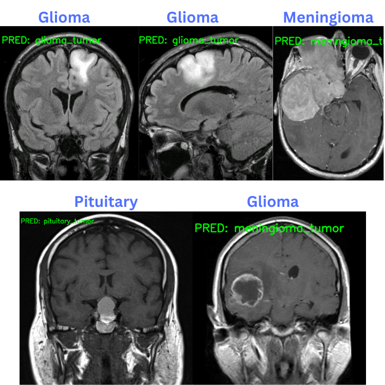
The model made only one mistake when it predicted the glioma tumor as meningioma tumor. All the other predictions are correct.

Vision Transformer Training on the CIFAR10 Dataset

Now, we will train the Vision Transformer model on the CIFAR10 dataset. The train_cifar10.py file contains the code for this. It is very similar to the previous training script. The only difference is that we load the dataset from torchvision.datasets instead of custom data loader.

Along with that we also apply the CIFAR10 AutoAugmentPolicy which applies more than 20 image augmentations to avoid overfitting. As we will see soon, getting high accuracy from scratch is still very difficult on the CIFAR10 dataset.

Let’s start the training.

python train_cifar10.py --learning-rate 0.0005 --num-layers 6 --num-heads 6 --embed-dim 288 --hidden-dim 1152 --epochs 50 --batch-size 128

In this case, we start with a learning rate of 0.0005. The model that we are building here is not the base model. We have a much smaller model with 6 transformer layers, 6 attention heads, and an embedding dimension of 288. The model will train for 50 epochs with a batch size of 128.

The above hyperparameters build a 6.2 million parameter model.

The following is the truncated output from the terminal.

[INFO]: Epoch 1 of 50
Training
100%|████████████████████████████████████████████████████████████████████████████████████████████████████████████████████████████████████████████████████████████████████████████| 391/391 [00:53<00:00,  7.35it/s]
Validation
100%|██████████████████████████████████████████████████████████████████████████████████████████████████████████████████████████████████████████████████████████████████████████████| 79/79 [00:04<00:00, 17.69it/s]
Training loss: 1.992, training acc: 27.050
Validation loss: 1.815, validation acc: 34.420

Best validation loss: 1.8151317789584775

Saving best model for epoch: 1

Adjusting learning rate of group 0 to 5.0000e-04.
--------------------------------------------------
.
.
.
[INFO]: Epoch 27 of 50
Training
100%|████████████████████████████████████████████████████████████████████████████████████████████████████████████████████████████████████████████████████████████████████████████| 391/391 [00:51<00:00,  7.65it/s]
Validation
100%|██████████████████████████████████████████████████████████████████████████████████████████████████████████████████████████████████████████████████████████████████████████████| 79/79 [00:04<00:00, 17.53it/s]
Training loss: 0.503, training acc: 82.662
Validation loss: 0.847, validation acc: 71.760

Best validation loss: 0.8466630374329

Saving best model for epoch: 27

Adjusting learning rate of group 0 to 5.0000e-05.
--------------------------------------------------
.
.
.
--------------------------------------------------
[INFO]: Epoch 50 of 50
Training
100%|████████████████████████████████████████████████████████████████████████████████████████████████████████████████████████████████████████████████████████████████████████████| 391/391 [00:51<00:00,  7.65it/s]
Validation
100%|██████████████████████████████████████████████████████████████████████████████████████████████████████████████████████████████████████████████████████████████████████████████| 79/79 [00:04<00:00, 17.25it/s]
Training loss: 0.322, training acc: 89.002
Validation loss: 0.916, validation acc: 73.660
Adjusting learning rate of group 0 to 5.0000e-06.
--------------------------------------------------
TRAINING COMPLETE

The model reached the best validation loss on epoch 27. After that, the loss kept on increasing.

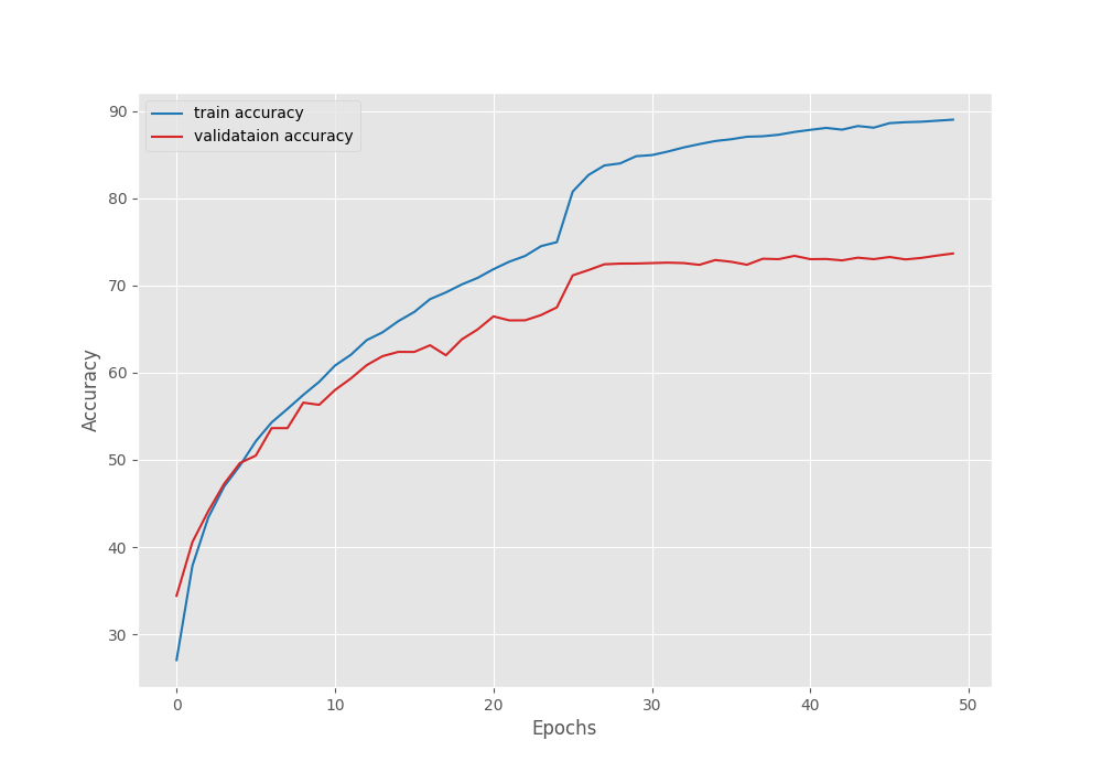
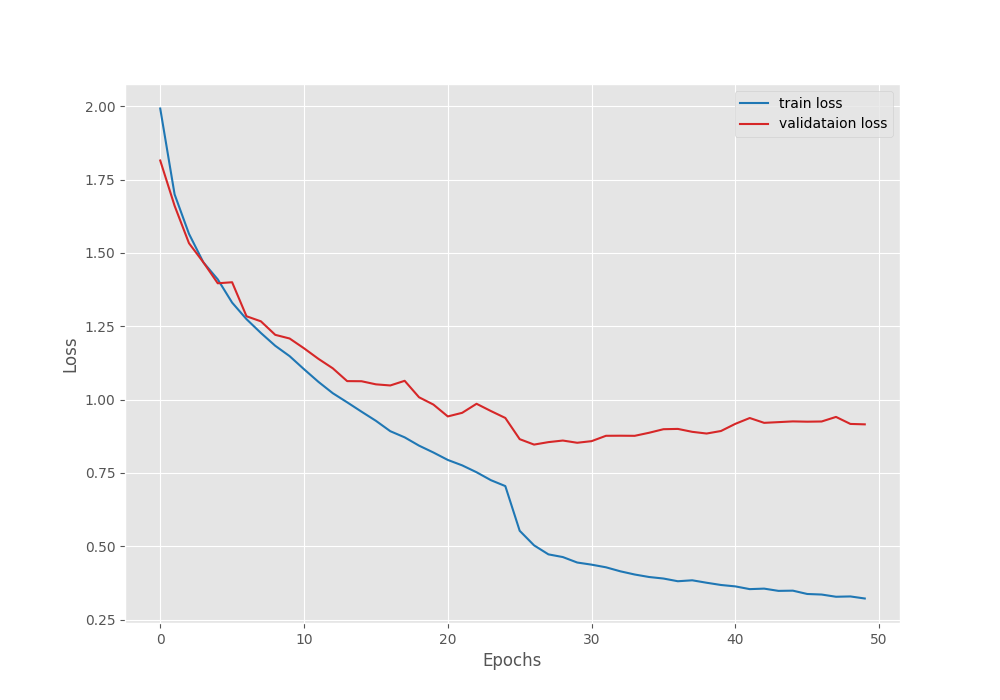
The above graph shows that the loss kept slowly increasing after epoch 27. Maybe if we decrease the learning a bit more aggressively, we may reach a lower loss by the end of training.

Inference using the CIFAR10 Trained Vision Transformer Model

For the final experiment, we will run inference using the best model weights from the CIFAR10 training.

python inference.py --num-layers 6 --num-heads 6 --embed-dim 288 --hidden-dim 1152 --weights ../outputs/cifar10/best_model.pth --input ../input/inference_data/cifar10/ --num-classes 10 --data cifar10

This time we need to be aware to pass the proper model hyperparameters or else the checkpoint weights cannot be loaded into the initialized model.

The following image shows the results.

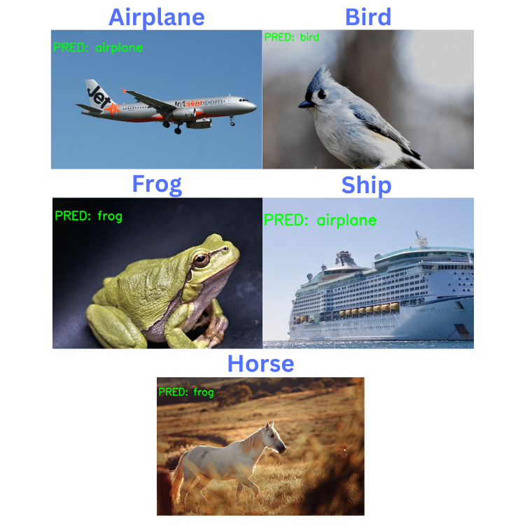
The model made two mistakes. In one instance, it is predicting the horse as a frog, and in another one, the ship as an airplane. This is expected as the best model weights had a validation accuracy of 71%.

To improve the results for both training experiments, we can also fine-tune a pretrained Vision Transformer [LINL TO Fine Tuning Vision Transformer and Visualizing Attention Maps] model.

Summary and Conclusion

In this article, we trained the Vision Transformer model from scratch using the PyTorch deep learning framework. We observed how challenging it can be to train transformer models from scratch. We also went through hyperparameter selection for training and model initialization which helps when training from scratch. I hope that this article was worth your time.

If you have any doubts, thoughts, or suggestions, please leave them in the comment section. I will surely address them.

You can contact me using the Contact section. You can also find me on LinkedIn, and Twitter.

Credits

Brain tumor inference images:

• glioma_1.jpg
• glioma_2.jpg, glioma_3.jpg
• pituitary_1.jpeg
• meningioma_1.jpg