Hyperparameter Tuning using Keras Tuner

In the past few posts, we have been covering hyperparameter tuning quite extensively. And from the results, it was quite clear that hyperparameter tuning, although computationally expensive, is quite helpful in finding the best model that we can. In all the previous tutorials, we use the PyTorch framework with the same dataset so that we can compare the results. Here, we will change the approach a bit. We will use TensorFlow as the framework of choice. And we will use Keras Tuner for hyperparameter tuning of our model built using TensorFlow.

Before moving ahead, if you wish to take a look at the previous tutorials, then you can visit the following links. Starting with the basic theory of hyperparameter tuning, to hands-on coding using PyTorch, Skorch, and Ray Tune, we cover a lot of topics.

• An Introduction to Hyperparameter Tuning in Deep Learning.
• Manual Hyperparameter Tuning in Deep Learning using PyTorch.
• Hyperparameter Search with PyTorch and Skorch.
• Hyperparameter Tuning with PyTorch and Ray Tune.

If you are completely new to hyperparameter tuning in deep learning, then the above posts will surely help.

Now, let’s take a look at what we will cover in this tutorial.

• We will start with a brief introduction to Keras Tuner.
• Then we will explore that dataset that we will use here. We will be changing the dataset compared to the previous tutorial to make things a bit more interesting.
• Moving on to the coding section, we will tune the parameters specific to the deep learning model. They are:
  • Number of units in the Dense layer.
  • And the learning rate.
  • Here, we will not tune the epochs and batch size as we did in the last tutorial.
• After running the script for hyperparameter tuning, we will analyze the results and discuss what further steps to take.

A Brief Introduction to Keras Tuner

Keras officially became a high-level API for TensorFlow with TensorFlow 2.0. Instead of importing it separately, now we can use tensorflow.keras to access all the modules.

With all this, Keras Tuner and its functionalities also became easily available. Although Keras Tuner still stands as a separate library, it is very closely integrated with TensorFlow and of course, Keras as well.

So, what is Keras Tuner?

KerasTuner is an easy-to-use, scalable hyperparameter optimization framework that solves the pain points of hyperparameter search. Easily configure your search space with a define-by-run syntax, then leverage one of the available search algorithms to find the best hyperparameter values for your models.

KerasTuner

Not only that, it contains a number of built-in search algorithms to make the search process even easier for us. We will get into more details of these a bit later.

Further on, when we get into the coding part of the tutorial, you will get to know all the details and how to deal with each part of the hyperparameter tuning process.

For now, you may take a look at the docs and get a bit more familiar with the coding style of Keras Tuner. Also, you need to install Keras Tuner on your machine if you wish to run all the code locally. You can visit the website to install it, or just execute the following command in the Anaconda or Python Virtual Environment of your choice.

pip install keras-tuner --upgrade

The Dataset

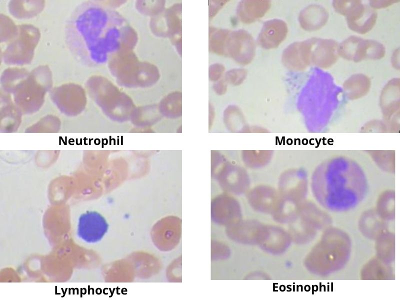
We will use the Blood Cell Images dataset from Kaggle for this project. This dataset contains images of blood cells categorized into four different cell types.

This dataset contains 12,500 augmented images of blood cells. The four classes are:

• Eosinophil
• Lymphocyte
• Monocyte
• Neutrophil

Here are a few images from the dataset with their corresponding classes.

This dataset contains just enough images to start our experiment with Keras Tuner. However, there are a few details that we should know about the dataset. If you download the dataset and extract it, you should see the following directory structure.

├── dataset2-master
│   └── dataset2-master
│       ├── images
│       │   ├── TEST
│       │   │   ├── EOSINOPHIL [623 entries exceeds filelimit, not opening dir]
│       │   │   ├── LYMPHOCYTE [620 entries exceeds filelimit, not opening dir]
│       │   │   ├── MONOCYTE [620 entries exceeds filelimit, not opening dir]
│       │   │   └── NEUTROPHIL [624 entries exceeds filelimit, not opening dir]
│       │   ├── TEST_SIMPLE
│       │   │   ├── EOSINOPHIL [13 entries exceeds filelimit, not opening dir]
│       │   │   ├── LYMPHOCYTE
│       │   │   ├── MONOCYTE
│       │   │   └── NEUTROPHIL [48 entries exceeds filelimit, not opening dir]
│       │   └── TRAIN
│       │       ├── EOSINOPHIL [2497 entries exceeds filelimit, not opening dir]
│       │       ├── LYMPHOCYTE [2483 entries exceeds filelimit, not opening dir]
│       │       ├── MONOCYTE [2478 entries exceeds filelimit, not opening dir]
│       │       └── NEUTROPHIL [2499 entries exceeds filelimit, not opening dir]
│       └── labels.csv
└── dataset-master
    └── dataset-master
        ├── Annotations [343 entries exceeds filelimit, not opening dir]
        ├── JPEGImages [366 entries exceeds filelimit, not opening dir]
        └── labels.csv 

We can see two folders, dataset2-master and dataset-master. We are interested in the dataset2-master folder. This contains the images divided into their respective class folders. We have the TRAIN, TEST, and TEST_SIMPLE folders.

For training, we will obviously use the TRAIN folder images which is around 10000 images in total. For validation, we have two options, TEST and TEST_SIMPLE. We will go with the TEST folder as it contains 2487 images. TEST_SIMPLE contains just above 70 images.

Before moving on to the next part, be sure to download the dataset to your machine. We will check out the directory structure in the next section.

The Directory Structure

The following block shows the directory structure for the project.

├── input
│   ├── dataset2-master
│   │   └── dataset2-master
│   │       ├── images
│   │       │   ├── TEST
│   │       │   │   ├── EOSINOPHIL [623 entries exceeds filelimit, not opening dir]
│   │       │   │   ├── LYMPHOCYTE [620 entries exceeds filelimit, not opening dir]
│   │       │   │   ├── MONOCYTE [620 entries exceeds filelimit, not opening dir]
│   │       │   │   └── NEUTROPHIL [624 entries exceeds filelimit, not opening dir]
│   │       │   ├── TEST_SIMPLE
│   │       │   │   ├── EOSINOPHIL [13 entries exceeds filelimit, not opening dir]
│   │       │   │   ├── LYMPHOCYTE
│   │       │   │   ├── MONOCYTE
│   │       │   │   └── NEUTROPHIL [48 entries exceeds filelimit, not opening dir]
│   │       │   └── TRAIN
│   │       │       ├── EOSINOPHIL [2497 entries exceeds filelimit, not opening dir]
│   │       │       ├── LYMPHOCYTE [2483 entries exceeds filelimit, not opening dir]
│   │       │       ├── MONOCYTE [2478 entries exceeds filelimit, not opening dir]
│   │       │       └── NEUTROPHIL [2499 entries exceeds filelimit, not opening dir]
│   │       └── labels.csv
│   ├── dataset-master
│   │   └── dataset-master
│   │       ├── Annotations [343 entries exceeds filelimit, not opening dir]
│   │       ├── JPEGImages [366 entries exceeds filelimit, not opening dir]
│   │       └── labels.csv
├── outputs
│   ├── best_model
│   ├── blood_cell_classification [7 entries exceeds filelimit, not opening dir]
│   ├── accuracy.png
│   └── loss.png
├── src
│   ├── model.py
│   ├── prepare_datasets.py
│   └── tune.py

• The input directory contains our dataset in the dataset2-master folder. We can ignore the dataset-master folder for this tutorial.
• The outputs directory will contain:
  • The hyperperarameter tuning results in the blood_cell_classification folder. This is the directory that is created by Keras Tuner to store all the results.
  • While doing the final training, we will save the best model in the best_model folder.
  • It will also contain the accuracy and loss graphs for the final training.
• And the src directory contains the Python files for which we will write the code.

You can download the zip file containing the Python files and the other folder with the correct structure. You just need to download the dataset if you intend the run the code locally,

Hyperparameter Tuning using Keras Tuner

Let’s start with the coding part of the tutorial. We have three Python files in which we will be writing the code.

Let’s start with the dataset preparation code.

Preparing the Blood Cell Images Dataset

Before we can start with the hyperparameter tuning process with Keras Tuner, we need to prepare the dataset. Here are the steps we are going to follow:

• Prepare the training and validation set for the hyperparameter search as well the training.
• Apply required augmentations to the images.
• Resize the images.
• Apply proper batch size. Neither too high, nor too low.

Thankfully, TensorFlow’s ImageDataGenerator class and its flow_from_directory() method will make things easy for us. And because the dataset is already divided into different folders for training and validation, it will be even simpler.

Let’s start writing the code in the prepare_datasets.py file.

The first code block contains the TensorFlow import and a few constants.

import tensorflow as tf

# Define the image shape to resize to.
IMAGE_SHAPE = (224, 224)
# Batch size.
BATCH_SIZE = 32
# Train folder path.
TRAINING_DATA_DIR = '../input/dataset2-master/dataset2-master/images/TRAIN'
# Validataion folder path.
VALID_DATA_DIR = '../input/dataset2-master/dataset2-master/images/TEST'

We will resize all the images to 224×224 dimensions. The batch size is going to be 32. And we define the path to the training and validation data folders as well in the above code block.

The next code block contains two functions:

• get_datagen(): This will create the training and validation data generators using the ImageDataGenerator class.
• get_data_batches(): To create the training and validation data batches using the flow_from_directory() method.

def get_datagen():
    train_datagen = tf.keras.preprocessing.image.ImageDataGenerator(
    rescale=1./255,
    horizontal_flip=True, 
    vertical_flip=True,
    rotation_range=40,
    zoom_range=0.3,
    shear_range=0.3,
    )
    valid_datagen = tf.keras.preprocessing.image.ImageDataGenerator(
    rescale=1./255,
    )
    return train_datagen, valid_datagen

def get_data_batches(train_datagen, valid_datagen):
    # Define the train data generator.
    train_batches = train_datagen.flow_from_directory(
        TRAINING_DATA_DIR,
        shuffle=True,
        target_size=IMAGE_SHAPE,
        seed=42,
        batch_size=BATCH_SIZE
    )
    # Define the validation data generator.
    valid_batches = valid_datagen.flow_from_directory(
        VALID_DATA_DIR,
        shuffle=False,
        target_size=IMAGE_SHAPE,
        seed=42,
        batch_size=BATCH_SIZE
    )
    return train_batches, valid_batches

While creating the data generators, first we are rescaling the images by dividing the pixels by 255.0. For the training image augmentation, we are applying:

• Horizontal and vertical flipping.
• Roatation of images by 40 degrees.
• Randomly zooming.
• And image shearing.

We are not applying any augmentation to the validation images, just rescaling the pixel values.

Coming to the get_data_batches() function. This accepts the training and validation data generators as parameters. Then it creates the data batches which contain both, the images, and the labels. We are applying a seed value, so that each time, the training and validation data will be in the same order. Also, note that we shuffle the training data batches only.

The Neural Network Model

This is an important part of the tutorial. Here, we will build the neural network model for which we will carry out the hyperparameter tuning.

The model-building process here is going to be a bit different compared to what we usually do in TensorFlow. We need to properly set the tunable parameters and because of that, the code will also change a bit.

Taking a look at the code and then going to the explanation will make things easier to understand. Let’s write the code in model.py file.

import tensorflow as tf

def build_model(hp):
    model = tf.keras.Sequential()
    model.add(tf.keras.layers.Conv2D(
        filters=32, kernel_size=(5, 5), activation='relu', 
        input_shape=(224, 224, 3)
    ))

    model.add(tf.keras.layers.Conv2D(
        filters=64, kernel_size=(3, 3), activation='relu'
    ))
    model.add(tf.keras.layers.BatchNormalization())
    model.add(tf.keras.layers.MaxPooling2D(pool_size=(2, 2), strides=2))
    model.add(tf.keras.layers.Conv2D(
        filters=128, kernel_size=(3, 3), activation='relu'
    ))
    model.add(tf.keras.layers.BatchNormalization())
    model.add(tf.keras.layers.MaxPooling2D(pool_size=(2, 2), strides=2))
    model.add(tf.keras.layers.Conv2D(
        filters=256, kernel_size=(3, 3), activation='relu'
    ))
    model.add(tf.keras.layers.BatchNormalization())

    model.add(tf.keras.layers.Flatten())
    # Tuning the number of units in the first Dense Layer,
    # values between 128 and 256.
    hp_units_1 = hp.Int('units_1', min_value=128, max_value=256, step=64)
    model.add(tf.keras.layers.Dense(units=hp_units_1, activation='relu'))
    # Add the final classification layer.
    model.add(tf.keras.layers.Dense(4))

    # Tune the learning rate for the optimizer
    # Choose an optimal value from 0.01, 0.001, or 0.0001
    hp_learning_rate = hp.Choice('learning_rate', values=[1e-2, 1e-3, 1e-4])

    model.compile(optimizer=tf.keras.optimizers.Adam(learning_rate=hp_learning_rate),
                loss=tf.keras.losses.CategoricalCrossentropy(from_logits=True),
                metrics=['accuracy'])
    return model

Explanation of the Neural Network Model

In the above code block, we have just one import, that tensorflow. All the important things are happening in the build_model() function.

The first thing to note is that it accepts an argument called hp. This is the instance of the Hyperparameter Tuning class that will actually help us choose the different parameters that we can tune.

Starting from lines 3 to 23, we build a model in a Sequential manner. This consists of stacking of 2D convolutional, Max-Pooling, and Batch Normalization layers. Here, there are no tunable hyperparameters.

Before moving on to the Dense layers, we flatten the features on line 25.

On line 28, we define hp_units_1 which will help select the best-required number of units for the next Dense layer. It is defined using hp.Int() method indicating that it can any value from 128 to 256 with a step size of 64. Also 'units_1' is a string defining the name of the tunable hyperparameter. We can use it to refer to this parameter later when needed. Among the model layer parameters, this is the only tunable one.

For the final layer Dense layer, we just define the number of classes that we have.

Then on line 35, we set the learning rate as one of the tunable parameters as well. The search algorithm will choose the best value from 0.01, 0.001, and 0.0001. This we are using while compiling the model.

Note that these hyperparameters will be chosen at random when the parameter search happens.

This is all we need for the neural network model. These two are all the parameters that we will be using for hyperparameter tuning using Keras Tuner.

The Tuning and Training Script

Now, we will move on to the final Python script. This is the script, which will do the hyperparameter search/tuning using Keras Tuner. It will try to find the best number of units for the Dense layer and the best learning rate as well.

This code will go into the tune.py script.

The first code block contains the import statements.

from prepare_datasets import (
    get_datagen, get_data_batches
)
from model import build_model

import tensorflow as tf
import matplotlib.pyplot as plt
import keras_tuner

plt.style.use('ggplot')

We import our own modules along with TensorFlow, and Keras Tuner.

Next, prepare the dataset to get the training and validation batches.

# Prepare the datasets.
train_datagen, valid_datagen = get_datagen()
train_batches, valid_batches = get_data_batches(
    train_datagen, valid_datagen
)

Initialize RandomSearch and Start the Hyperparameter Search

The next part of the code is important. This is where we will instantiate the RandomSearch algorithm from keras_tuner. Then we will start the hyperparameter search.

# Instantiate RandomSearch from Keras Tuner.
tuner = keras_tuner.RandomSearch(
    build_model,
    objective='val_accuracy',
    max_trials=10,
    directory='../outputs/',
    project_name='blood_cell_classification'
)

# Instead of tuning the number of epochs, we use Early Stopping.
early_stopping = tf.keras.callbacks.EarlyStopping(monitor='val_loss', patience=3)

# Start the hyperparameter search for the model.
tuner.search(
    train_batches,
    validation_data=valid_batches, 
    epochs=10, 
    callbacks=[early_stopping],
)

The tuner variable holds the object of RandomSearch. Let’s go through the important arguments.

• First pass the build_model() model that we defined in the model.py file. Note that this function automatically accepts the hyperparameter object as the parameter that we observed earlier. That has the hp parameter in that function.
• Next, is the objective. It is a string here defined by 'val_accuracy', which means that the best hyperparameters will be judged by the highest validation accuracy.
• max_trials is 10. This is the number of hyperparameter searches to perform. If you are running this locally, provide this value by considering your hardware as well. This might even take a few hours to run through.
• The directory stores the hyperparameter information in JSON files and the checkpoints for each trial.
• The project_name is the additional directory that keras_tuner automatically creates to store the above results.

We are not tuning the number of epochs here. So, we create an EarlyStopping callback to stop the search process when the validation loss does not improve for 3 epochs.

Next, we start the hyperparameter search using the search() method. We provide the training batches, the validation batches, the number of epochs, and the callbacks. Essentially, the search() method can accept all the arguments that the fit() method from Keras accepts.

Get the Best Hyperparameters

After the hyperparameter search is complete, we need to extract the best hyperparameters and train the model final time.

# Get the best hyperparameters.
best_hps=tuner.get_best_hyperparameters(num_trials=1)[0]

print(f"""
Units for first densely-connected layer: {best_hps.get('units_1')} 
Optimal learning rate for the optimizer: {best_hps.get('learning_rate')}.
""")

# Train the model one final time while saving the best model.
save_best = tf.keras.callbacks.ModelCheckpoint(
    filepath='../outputs/best_model/',
    monitor='val_loss',
    save_best=True,
    verbose=1
)
model = tuner.hypermodel.build(best_hps)
history = model.fit(
    train_batches, 
    validation_data=valid_batches, 
    epochs=50,
    callbacks=[early_stopping, save_best],
    workers=4,
    use_multiprocessing=True
)

We can get the best hyperparameters using tuner.get_best_hyperparameters(). This we store in the best_hps variable.

Before starting the training, we initialize ModelCheckpoint class to save the best checkpoints to disk.

On line 50, we create the model again using the best hyperparameters and start the training. We train for 50 epochs using the callbacks for early stopping and for saving the best model.

After the training is complete, one final thing is left. We need to plot the loss and accuracy graphs and save them to disk.

train_loss = history.history['loss']
train_acc = history.history['accuracy']
valid_loss = history.history['val_loss']
valid_acc = history.history['val_accuracy']
# Function to save the loss and accuracy graphs.
def save_plots(train_acc, valid_acc, train_loss, valid_loss):
    """
    Function to save the loss and accuracy plots to disk.
    """
    # Accuracy plots.
    plt.figure(figsize=(12, 9))
    plt.plot(
        train_acc, color='green', linestyle='-', 
        label='train accuracy'
    )
    plt.plot(
        valid_acc, color='blue', linestyle='-', 
        label='validataion accuracy'
    )
    plt.xlabel('Epochs')
    plt.ylabel('Accuracy')
    plt.legend()
    plt.savefig('../outputs/accuracy.png')
    plt.show()
    # Loss plots
    plt.figure(figsize=(12, 9))
    plt.plot(
        train_loss, color='orange', linestyle='-', 
        label='train loss'
    )
    plt.plot(
        valid_loss, color='red', linestyle='-', 
        label='validataion loss'
    )
    plt.xlabel('Epochs')
    plt.ylabel('Loss')
    plt.legend()
    plt.savefig('../outputs/loss.png')
    plt.show()

save_plots(train_acc, valid_acc, train_loss, valid_loss)

The plots are saved to the outputs folder.

This is all the code we need for this tutorial. In the next section, we will execute the script and analyze the results.

Executing tune.py

You can open your command line/terminal inside the src directory and execute the following command if you wish to run this on your local system.

python tune.py 

The following block shows the sample output.

Found 9957 images belonging to 4 classes.
Found 2487 images belonging to 4 classes.
Search: Running Trial #1

Hyperparameter    |Value             |Best Value So Far 
units_1           |128               |?                 
learning_rate     |0.0001            |?                 

2021-12-08 16:41:58.669330: I tensorflow/compiler/mlir/mlir_graph_optimization_pass.cc:185] None of the MLIR Optimization Passes are enabled (registered 2)
Epoch 1/10
312/312 [==============================] - 64s 196ms/step - loss: 1.5519 - accuracy: 0.3232 - val_loss: 1.3863 - val_accuracy: 0.2509
Epoch 2/10
312/312 [==============================] - 62s 199ms/step - loss: 1.1867 - accuracy: 0.4390 - val_loss: 10.9274 - val_accuracy: 0.2585
Epoch 3/10
312/312 [==============================] - 60s 193ms/step - loss: 1.0148 - accuracy: 0.5726 - val_loss: 56.4004 - val_accuracy: 0.2754
Epoch 4/10
312/312 [==============================] - 61s 197ms/step - loss: 0.8928 - accuracy: 0.6348 - val_loss: 79.7832 - val_accuracy: 0.2541
Trial 1 Complete [00h 04m 15s]
val_accuracy: 0.2754322588443756

Best val_accuracy So Far: 0.2754322588443756
Total elapsed time: 00h 04m 15s

Search: Running Trial #2

Hyperparameter    |Value             |Best Value So Far 
units_1           |128               |128               
learning_rate     |0.01              |0.0001            

Epoch 1/10
312/312 [==============================] - 63s 202ms/step - loss: 17.9435 - accuracy: 0.2491 - val_loss: 1.3865 - val_accuracy: 0.2509
Epoch 2/10
312/312 [==============================] - 63s 201ms/step - loss: 1.3985 - accuracy: 0.2466 - val_loss: 1.3871 - val_accuracy: 0.2493
Epoch 3/10
312/312 [==============================] - 62s 200ms/step - loss: 1.4076 - accuracy: 0.2419 - val_loss: 1.3976 - val_accuracy: 0.2489
Epoch 4/10
312/312 [==============================] - 64s 206ms/step - loss: 1.4531 - accuracy: 0.2476 - val_loss: 1.3871 - val_accuracy: 0.2493
Trial 2 Complete [00h 04m 14s]
val_accuracy: 0.25090470910072327

Best val_accuracy So Far: 0.2754322588443756
Total elapsed time: 00h 08m 30s


Search: Running Trial #7

Hyperparameter    |Value             |Best Value So Far 
units_1           |128               |192               
learning_rate     |0.001             |0.0001            

Epoch 1/10
312/312 [==============================] - 61s 193ms/step - loss: 2.4017 - accuracy: 0.2441 - val_loss: 1.3863 - val_accuracy: 0.2493
Epoch 2/10
312/312 [==============================] - 60s 192ms/step - loss: 1.4140 - accuracy: 0.2431 - val_loss: 39.6047 - val_accuracy: 0.2509
Epoch 3/10
312/312 [==============================] - 61s 195ms/step - loss: 1.4015 - accuracy: 0.2454 - val_loss: 58.6821 - val_accuracy: 0.2485
Epoch 4/10
312/312 [==============================] - 61s 194ms/step - loss: 1.4160 - accuracy: 0.2470 - val_loss: 44.5201 - val_accuracy: 0.2477
Trial 7 Complete [00h 04m 06s]
val_accuracy: 0.25090470910072327

Best val_accuracy So Far: 0.41013267636299133
Total elapsed time: 00h 35m 02s

Units for first densely-connected layer: 192 
Optimal learning rate for the optimizer: 0.0001.

Epoch 1/50
312/312 [==============================] - 21s 65ms/step - loss: 1.4890 - accuracy: 0.4010 - val_loss: 1.3855 - val_accuracy: 0.2927

Epoch 00001: saving model to ../outputs/best_model/
2021-12-08 17:17:22.650113: W tensorflow/python/util/util.cc:348] Sets are not currently considered sequences, but this may change in the future, so consider avoiding using them.
Epoch 2/50
312/312 [==============================] - 21s 66ms/step - loss: 0.9554 - accuracy: 0.5780 - val_loss: 3.4908 - val_accuracy: 0.2646

Epoch 00002: saving model to ../outputs/best_model/
Epoch 3/50
312/312 [==============================] - 21s 67ms/step - loss: 0.7720 - accuracy: 0.6723 - val_loss: 1.3853 - val_accuracy: 0.5726

Epoch 00003: saving model to ../outputs/best_model/
Epoch 4/50
312/312 [==============================] - 21s 67ms/step - loss: 0.6045 - accuracy: 0.7581 - val_loss: 7.4867 - val_accuracy: 0.4934

Epoch 00004: saving model to ../outputs/best_model/
Epoch 5/50
312/312 [==============================] - 21s 67ms/step - loss: 0.5349 - accuracy: 0.7864 - val_loss: 136.1895 - val_accuracy: 0.2497

Epoch 00005: saving model to ../outputs/best_model/
Epoch 6/50
312/312 [==============================] - 21s 67ms/step - loss: 0.4449 - accuracy: 0.8268 - val_loss: 13.3980 - val_accuracy: 0.4544

Epoch 00006: saving model to ../outputs/best_model/
 

As we can see, the search for the best hyperparameter started with units_1 set to 128 and learning_rate set to 0.0001. The search did not go for 10 trials, most probably because the hyperparameter search space did not amount to 10 different sets of hyperparameters. By the end of the search, we have the best Dense layer units of 192 and the best learning rate of 0.0001. Also, the entire search took somewhere around 35 minutes.

We can see the final training results with the best hyperparameters as well. Due to early stopping, the training ended after 6 epochs. Although the training accuracy and loss look pretty stable, the validation accuracy and loss seem unstable.

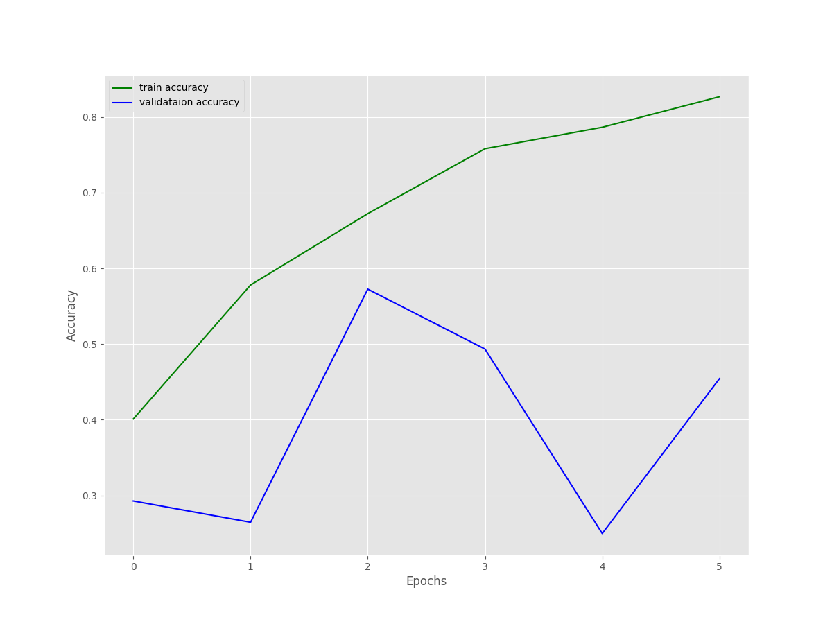
We can infer the same from the above accuracy and loss figures as well.

There could be several reasons for this.

• Firstly, maybe our search space was not good enough. Most probably, a wider range of values for the Dense layer and learning rate would help.
• Secondly, with increasing the values for the search space, we can try to run more number of trails.
• Also, working with medical imaging in deep learning can be difficult sometimes if we do not know what we are doing. The results are not always as we expect.
• And finally, maybe a deeper network with more convolutional layers and dense layers would help.

We can experiment with all of the above. But it is bound to take a lot of time and computational resources as well. If you try these, then letting others know in the comment section would surely help.

Summary and Conclusion

In this tutorial, you learned how to use Keras Tuner for hyperparameter tuning in deep learning. We started with a short introduction to Keras Tuner and moved on to the implementation. Although our results were not as good, they still gave us some insights into the pipeline of Keras Tuner. I hope that this tutorial was helpful to you.

If you have any doubts, thoughts, or suggestions, please leave them in the comment section. I will surely address them.

You can contact me using the Contact section. You can also find me on LinkedIn, and Twitter.