Hyperparameter Tuning with PyTorch and Ray Tune

In this tutorial, you will learn how to use Ray Tune for Hyperparameter Tuning in PyTorch. Finding the right hyperparameters is quite important to build a very good model for solving the deep learning problem we have at hand. In most situations, experience in training deep learning models can play a crucial role in choosing the right hyperparameters. But there will be a few situations where we need to employ some extra tools. Ray Tune is one such tool that we can use to find the best hyperparameters for our deep learning models in PyTorch. We will be exploring Ray Tune in depth in this tutorial, and writing the code to tune the hyperparameters of a PyTorch model.

If you are new to hyperparameter tuning or hyperparameter search in deep learning, you may find the following tutorials helpful.

• An Introduction to Hyperparameter Tuning in Deep Learning.
• Manual Hyperparameter Tuning in Deep Learning using PyTorch.
• Hyperparameter Search with PyTorch and Skorch.

In this tutorial, we will go one step further for hyperparameter tuning in deep learning. We will use Ray Tune which happens to be one of the best tools for this.

Topics to Cover

Let’s check out the points that we will cover in this tutorial:

• We will start with a short introduction to Ray Tune. In that we will cover:
  • What is Ray Tune?
  • What are the obvious disadvantages of using Skorch for hyperparamter tuning/search that we faced in the last tutorial?
  • The solutions that Ray Tune provides to overcome the disadvantage of Skorch.
  • Installing Ray Tune locally.
• Then we will explore the dataset in short that we will use in this tutorial (It is the same dataset as in the last two tutorials).
• Next, we will move over to the coding part of the tutorial. We will try to get into as much depth of the code as possible.
• After the experiment, we will analyze the results along with visualizing the TensorBoard logs.
• We will discuss a few possible next steps to take to learn even more about the working of Ray Tune. You will also get access to a bonus Kaggle notebook which use a different dataset.
• Finally, we will end with a short conclusion to the post.

A Short Introduction to Ray Tune

Ray Tune is part of the Ray (Ray Core) project. Ray provides an API for building distributed applications distributed.

But we are most interested in Ray Tune which is a Python library for scalable hyperparameter tuning.

Although we will be using Ray Tune for hyperparameter tuning with PyTorch here, it is not limited to only PyTorch. In fact, the following points from the official website summarize its wide range of capabilities quite well.

1. Launch a multi-node distributed hyperparameter sweep in less than 10 lines of code.

2. Supports any machine learning framework, including PyTorch, XGBoost, MXNet, and Keras.

3. Automatically manages checkpoints and logging to TensorBoard.

4. Choose among state of the art algorithms such as Population Based Training (PBT), BayesOptSearch, HyperBand/ASHA.

5. Move your models from training to serving on the same infrastructure with Ray Serve.

Ray Tune

As we can see, it has support for multiple deep learning frameworks, automatic checkpointing and TensorBoard logging, and even different algorithms for hyperparameter search. You will get to experience a lot of these in this tutorial.

A Few Disadvantages of Skorch

In the last tutorial, we did a hyperparameter search using the Skorch library. Although it was quite helpful, there were a few disadvantages.

• We could not use GPU while carrying out the hyperparameter search. Or at least, it is not just as easy to use a GPU with Skorch and PyTorch for hyperparameter search and tuning. And we know how crucial it is to speed up computations in deep learning with the use of a GPU.
• And even more so when we want to run a number of different searches to solve a problem. If you remember or go through the previous tutorial, then you will know that we were not able to run the search by training on the entire dataset because it was very time-consuming. We were only running the search on a few batches of data.
• We performed Grid Search which by now we know is not the best method. Random Search is much better than Grid Search for Hyperparameter Tuning.

That changes with this tutorial. We will use Ray Tune along with PyTorch for hyperparameter tuning. The integration between the two is quite good. The following are a few of the advantageous points that we will experience:

• Will be able to use a GPU while searching for the best hyperparameters.
• This means that we will also be able to run the search on the entire dataset.
• Ray Tune does automatic checkpointing and TensorBoard logging. We need not save the chechkpoints or the accuracy and loss plots manually as we did with Skorch.
• Ray Tune is even capable of running multiple search experiments on a single GPU if the GPU memory allows it.
• And we will be performing Random Search instead of Grid Search using Ray Tune.

The above are really some very compelling reasons to learn and try out Ray Tune. Before using it, let’s install it first.

Install Ray Tune

Ray has integration with a few other dependencies as well. But we need to install Ray with Tune. In your Anaconda or Python virtual environment of choice, execute the following command.

pip install -U ray[tune]

Let the installation complete and you are good to go.

Other Libraries that We Need…

This tutorial also needs PyTorch. All the code has been developed, run, and tested with PyTorch 1.10 (latest at the time of writing this). To install PyTorch in your system head over to the official site and choose the build according to your environment.

Dataset for the Tutorial

We will use the same dataset as we did in the last two tutorials.

That is the Natural Images from Kaggle with 8 classes: airplane, car, cat, dog, flower, fruit, motorbike, person. It has a total of 6899 images.

The main reason is that in each post we are trying to improve upon the methods of the previous post. And unless we use the same dataset we will not be able to compare the results.

To avoid the process of dataset selection being monotonous, you will also get access to a Kaggle notebook at the end of the tutorial that uses a different dataset with PyTorch and Ray Tune for hyperparameter tuning.

For now, you can download the dataset from here. 

The Directory Structure

Let’s check out the directory structure for this tutorial.

├── input
│   └── natural_images
│       ├── airplane [727 entries exceeds filelimit, not opening dir]
│       ├── car [968 entries exceeds filelimit, not opening dir]
│       ├── cat [885 entries exceeds filelimit, not opening dir]
│       ├── dog [702 entries exceeds filelimit, not opening dir]
│       ├── flower [843 entries exceeds filelimit, not opening dir]
│       ├── fruit [1000 entries exceeds filelimit, not opening dir]
│       ├── motorbike [788 entries exceeds filelimit, not opening dir]
│       └── person [986 entries exceeds filelimit, not opening dir]
├── outputs
│   └── raytune_result
│       └── train_and_validate_2021-12-02_08-21-49 [22 entries exceeds filelimit, not opening dir]
└── src
    ├── config.py
    ├── datasets.py
    ├── model.py
    ├── search_and_train.py
    └── train_utils.py

• The input folder contains the dataset directory.
• The outputs folder will contain all the results from the hyperparameter search. This includes the checkpoints for different runs, the best hyperparameter, and even the TensorBoard logs.
• Finally, we five Python files in the src folder. We will get into the details of these in the coding section of the tutorial.

Downloading the zip file for this tutorial will give you access to the source code and the directory structure. You just need to download the dataset and set it up as needed.

Hyperparameter Tuning with PyTorch and Ray Tune

From this section onward, we will start with the coding part of the tutorial. As there are 5 Python files, we will tackle them in the following order:

• config.py
• train_utils.py
• datasets.py
• model.py
• search_and_train.py

We will try to keep the code as modular as possible. So, if you would like to edit the code in the future, you can do it easily.

The Configuration File

The configuration file will hold the training parameters, constants for the dataset preparation, scheduler settings for Ray Tune, and search settings for Ray Tune.

The following code block contains the content that will go into config.py file.

import os

# Training parameters.
EPOCHS = 50
# Data root.
DATA_ROOT_DIR = os.path.abspath('../input/natural_images')
# Number of parallel processes for data fetching.
NUM_WORKERS = 4
# Ratio of split to use for validation.
VALID_SPLIT = 0.1
# Image to resize to in tranforms.
IMAGE_SIZE = 224

# For ASHA scheduler in Ray Tune.
MAX_NUM_EPOCHS = 50
GRACE_PERIOD = 1

# For search run (Ray Tune settings).
CPU = 1
GPU = 1
# Number of random search experiments to run.
NUM_SAMPLES = 20

Here, we have just one import, that is the os module.

For the model training parameters we have:

• Number of epochs to train for equal, to 50.
• The root path to the data directory. You may notice that it is enclosed within the abspath function. Without this, I was facing, FileNotNoundError, although there is nothing wrong with the path or the data folder. This must have something to do with the multi-processing that Ray Tune uses. Still, I am not quite sure but this solves the issue. They use the same technique in one of the official tutorials, so, we can safely use this.
• We are using 4 processes for the data preparation which will fasten up the process of DataLoader and transforms in PyTorch.
• Just like the previous tutorials, we use 10% of the data for validation.
• The images are resized to 224×224 dimensions.

Then we have the settings for the Ray Tune ASHAScheduler which stands for AsyncHyperBandScheduler. This is one of the easiest scheduling techniques to start with for hyperparameter tuning in Ray Tune. Let’s take a look at the setting (these are the parameters for the scheduler). Note that the actual parameter names are different and these are just constant names we are defining corresponding to those settings that we can import. You will see the actual parameter names in search_and_run.py where we define the scheduler.

• MAX_NUM_EPOCHS: Even though we have EPOCHS as 50, the scheduler can choose to stop any experiment that is within the MAX_NUM_EPOCHS, which is 50 as well. This means that an experiment might run for 20 epochs, or 30 epochs, or even the complete 50 epochs. And if the search experiment with the corresponding hyperparameters are not going well, then the scheduler will terminate the experiment.
• GRACE_PERIOD: Here the value is 1. This will ensure that even if the search with a particular set of hyperparameters is not going well, do not terminate the experiment if at least GRACE_PERIOD number of epochs have not passed for that experiment. So, when an experiment is not going well, and it has completed at least one epoch, then the scheduler will terminate it. We will see few such cases when running the experiment.

Next, we have the settings for the hyperparameter search in Ray Tune. Note that the actual parameter names are different and these are just constant names we are defining corresponding to those settings that we can import. You will see the actual parameter names in search_and_run.py where we define the run() method.

• CPU: Number of processors to use for each search. If you have access to a multi-core processor, you can set this to one for each experiment. And potentially, Ray Tune will be able to run multiple search experiments at a time.
• GPU: This is the number of GPUs to use for each search experiment. And it is an interestng one actually. You can also give a fractional number like 0.5 to this setting. This will actually divide you entire GPU memory in half and try to fit two search experiments within each half. So, if you have 10 GB of GPU memory, a value of 0.5, will try to alloctate around 5 GB for two experiments simulataneously. This will speed up the search process by a lot. But there is a catch to this. You need to ensure that according to the batch size and model parameters, all experiments will fit within the 5 GB of memory, else that particular search will error out.

If you have doubts about any of the above Ray Tune settings, do not worry. Things will become clear in search_and_train.py.

Prepare the Dataset

The dataset preparation code is almost similar to the previous tutorial.

The code here will go into the datasets.py file.

Starting with the imports and the training and validation transforms.

import torch

from torch.utils.data import DataLoader, Subset
from torchvision import datasets, transforms

# Training transforms
def get_train_transform(IMAGE_SIZE):
    train_transform = transforms.Compose([
        transforms.Resize((IMAGE_SIZE, IMAGE_SIZE)),
        transforms.ToTensor(),
        transforms.Normalize(
            mean=[0.5, 0.5, 0.5],
            std=[0.5, 0.5, 0.5]
        )
    ])
    return train_transform


# Validation transforms
def get_valid_transform(IMAGE_SIZE):
    valid_transform = transforms.Compose([
        transforms.Resize((IMAGE_SIZE, IMAGE_SIZE)),
        transforms.ToTensor(),
        transforms.Normalize(
            mean=[0.5, 0.5, 0.5],
            std=[0.5, 0.5, 0.5]
        )
    ])
    return valid_transform

This part is exactly the same as in the previous tutorial. We are not using any augmentation. We are just resizing the image according to the resize configuration that will be passed to the respective functions when creating the datasets.

Next, the functions to create the datasets and data loaders.

# Initial entire datasets,
# same for the entire and test dataset.
def get_datasets(IMAGE_SIZE, ROOT_DIR, VALID_SPLIT):
    dataset = datasets.ImageFolder(ROOT_DIR, transform=get_train_transform(IMAGE_SIZE))
    dataset_test = datasets.ImageFolder(ROOT_DIR, transform=get_valid_transform(IMAGE_SIZE))
    print(f"Classes: {dataset.classes}")
    dataset_size = len(dataset)
    print(f"Total number of images: {dataset_size}")

    valid_size = int(VALID_SPLIT*dataset_size)

    # Training and validation sets
    indices = torch.randperm(len(dataset)).tolist()
    dataset_train = Subset(dataset, indices[:-valid_size])
    dataset_valid = Subset(dataset_test, indices[-valid_size:])

    print(f"Total training images: {len(dataset_train)}")
    print(f"Total valid_images: {len(dataset_valid)}")
    return dataset_train, dataset_valid, dataset.classes


# Training and validation data loaders.
def get_data_loaders(
    IMAGE_SIZE, ROOT_DIR, VALID_SPLIT, BATCH_SIZE, NUM_WORKERS
):
    dataset_train, dataset_valid, dataset_classes = get_datasets(
        IMAGE_SIZE, ROOT_DIR, VALID_SPLIT
    )
    train_loader = DataLoader(
        dataset_train, batch_size=BATCH_SIZE, shuffle=True, num_workers=NUM_WORKERS
    )
    valid_loader = DataLoader(
        dataset_valid, batch_size=BATCH_SIZE, shuffle=False, num_workers=NUM_WORKERS
    )
    return train_loader, valid_loader, dataset_classes 

The get_datasets() function prepares the training and validation dataset. It also returns the class names at the end.

We will be calling the get_data_loaders() function from the executable script (search_and_train.py) while providing all the required arguments. This function calls the get_datasets() function and passes the required arguments to it. The data loader preparation function returns the training and validation data loaders along with the class names.

The Training Utils

We have two functions for the training utils. Those are the training and validation functions. We will keep them separate from the executable script so that the code remains as clean and modular as possible. Any changes to these functions should not affect the other parts of the code. These should calculate the loss and accuracy for each epoch and return them only.

The code will go into the train_utils.py file.

The training function.

import torch

# Training function.
def train(model, data_loader, optimizer, criterion, device):
    model.train()
    print('Training')
    train_running_loss = 0.0
    train_running_correct = 0
    counter = 0
    for i, data in enumerate(data_loader):
        counter += 1
        image, labels = data
        image = image.to(device)
        labels = labels.to(device)
        optimizer.zero_grad()
        # Forward pass.
        outputs = model(image)
        # Calculate the loss.
        loss = criterion(outputs, labels)
        train_running_loss += loss.item()
        # Calculate the accuracy.
        _, preds = torch.max(outputs.data, 1)
        train_running_correct += (preds == labels).sum().item()
        # Backpropagation.
        loss.backward()
        # Update the optimizer parameters.
        optimizer.step()
    
    # Loss and accuracy for the complete epoch.
    epoch_loss = train_running_loss / counter
    epoch_acc = 100. * (train_running_correct / len(data_loader.dataset))
    return epoch_loss, epoch_acc

The validation function.

# Validation function.
def validate(model, data_loader, criterion, device):
    model.eval()
    print('Validation')
    valid_running_loss = 0.0
    valid_running_correct = 0
    counter = 0
    
    with torch.no_grad():
        for i, data in enumerate(data_loader):
            counter += 1
            
            image, labels = data
            image = image.to(device)
            labels = labels.to(device)
            # Forward pass.
            outputs = model(image)
            # Calculate the loss.
            loss = criterion(outputs, labels)
            valid_running_loss += loss.item()
            # Calculate the accuracy.
            _, preds = torch.max(outputs.data, 1)
            valid_running_correct += (preds == labels).sum().item()
        
    # Loss and accuracy for the complete epoch.
    epoch_loss = valid_running_loss / counter
    epoch_acc = 100. * (valid_running_correct / len(data_loader.dataset))
    return epoch_loss, epoch_acc

The above two are very general training and validation functions for image classification. Also, these two are exactly the same as we had in the previous tutorial. Both of them calculate the loss and accuracy for each epoch and return them.

We just need to keep in mind that the training function does the backpropagation and parameter update which we do not need in the validation function.

The Neural Network Model

There is no change to the neural network model as well compared to the previous tutorial. Let’s write the code for that in model.py.

import torch.nn as nn
import torch.nn.functional as F
import torch

class CustomNet(nn.Module):
    def __init__(self, first_conv_out=16, first_fc_out=128):
        super().__init__()

        self.first_conv_out = first_conv_out
        self.first_fc_out = first_fc_out

        # All Conv layers.
        self.conv1 = nn.Conv2d(3, self.first_conv_out, 5)
        self.conv2 = nn.Conv2d(self.first_conv_out, self.first_conv_out*2, 3)
        self.conv3 = nn.Conv2d(self.first_conv_out*2, self.first_conv_out*4, 3)
        self.conv4 = nn.Conv2d(self.first_conv_out*4, self.first_conv_out*8, 3)
        self.conv5 = nn.Conv2d(self.first_conv_out*8, self.first_conv_out*16, 3)

        # All fully connected layers.
        self.fc1 = nn.Linear(self.first_conv_out*16, self.first_fc_out)
        self.fc2 = nn.Linear(self.first_fc_out, self.first_fc_out//2)
        self.fc3 = nn.Linear(self.first_fc_out//2, 8)

        # Max pooling layers
        self.pool = nn.MaxPool2d(2, 2)

    def forward(self, x):    
        # Passing though convolutions.
        x = self.pool(F.relu(self.conv1(x)))
        x = self.pool(F.relu(self.conv2(x)))
        x = self.pool(F.relu(self.conv3(x)))
        x = self.pool(F.relu(self.conv4(x)))
        x = self.pool(F.relu(self.conv5(x)))

        # Flatten.
        bs, _, _, _ = x.shape
        x = F.adaptive_avg_pool2d(x, 1).reshape(bs, -1)
        x = F.relu(self.fc1(x))
        x = F.relu(self.fc2(x))
        x = self.fc3(x)
        return x

if __name__ == '__main__':
    model = CustomNet(32, 512)
    tensor = torch.randn(1, 3, 224, 224)
    output = model(tensor)
    print(output.shape)

We have the same CustomNet() class. The model has two searchable parameters:

• first_conv_out: The output channels of the first convolutional layer. After that, the output channels keep on doubling
• first_fc_out: The output features of the first fully connected layer. Then the second fully connected layer halves the output features.

One other common way to describe the searchable parameters while building a neural network model is to completely define the convolutional layers manually. Then keep the number of output features of the fully connected layers as the hyperparameters. But we are following a bit of a different approach here.

The Search and Training Script

Now, we will write the code for the final executable script.

Here, all the code will go into the search_and_train.py file. This will contain:

• A train_and_validate() function that will prepare the data loaders and run the training and validation loops for the required number of epochs.
• A run_search() function that will set the Ray Tune’s search algorithm and scheduler and start the hyperparameter search.

Let’s start with the import statements.

from train_utils import train, validate
from model import CustomNet
from datasets import get_data_loaders
from config import (
    MAX_NUM_EPOCHS, GRACE_PERIOD, EPOCHS, CPU, GPU,
    NUM_SAMPLES, DATA_ROOT_DIR, NUM_WORKERS, IMAGE_SIZE, VALID_SPLIT
)

from ray import tune
from ray.tune import CLIReporter
from ray.tune.schedulers import ASHAScheduler

import torch
import torch.nn as nn
import numpy as np
import torch.optim as optim
import os

• Lines 1 to 5 contain the imports from our own modules and classes.
• From line 9, we have the ray and ray.tune imports:
  • The CLIReporter is the one that will output the required metrics on the terminal after each epoch.
  • And tune is used to set the ASHAScheduler scheduler and start the hyperparameter search. You will get to know the details as we code further.
• Then we have the imports for the torch modules.

The train_and_validate() Function

Next, we will define the train_and_validate() function. This prepares the data loaders, and execute the train() and validate() functions for the required number of epochs. After each epoch, it will pass down the validation loss and accuracy to the CLIReporter.

The following code block contains the entire function.

def train_and_validate(config):
    # Get the data loaders.
    train_loader, valid_loader, dataset_classes = get_data_loaders(
        IMAGE_SIZE, DATA_ROOT_DIR, VALID_SPLIT,
        config['batch_size'], NUM_WORKERS
    )

    device = torch.device('cuda:0' if torch.cuda.is_available() else 'cpu')
    # Initialize the model.
    model = CustomNet(
        config['first_conv_out'], config['first_fc_out']
    ).to(device)

    # Loss Function
    criterion = nn.CrossEntropyLoss()
    # Optimizer
    optimizer = optim.SGD(
        model.parameters(), lr=config['lr'], momentum=0.9
    )

    # Start the training.
    for epoch in range(EPOCHS):
        print(f"[INFO]: Epoch {epoch+1} of {EPOCHS}")
        train_epoch_loss, train_epoch_acc = train(
            model, train_loader, optimizer, criterion, device
        )
        valid_epoch_loss, valid_epoch_acc = validate(
            model, valid_loader, criterion, device
        )
  
        print(f"Training loss: {train_epoch_loss:.3f}, training acc: {train_epoch_acc:.3f}")
        print(f"Validation loss: {valid_epoch_loss:.3f}, validation acc: {valid_epoch_acc:.3f}")
        print('-'*50)

        with tune.checkpoint_dir(epoch) as checkpoint_dir:
            path = os.path.join(checkpoint_dir, 'checkpoint')
            torch.save((model.state_dict(), optimizer.state_dict()), path)
        tune.report(
            loss=valid_epoch_loss, accuracy=valid_epoch_acc
        )

Let’s check out the important bits of the above code block:

• On line 20, we get the data loaders.

Note that the batch size is according to the config dictionary. We will get to see the configuration settings a bit later when we define the run_search() function. For now, let’s keep in mind that the config dictionary holds the values for batch_size, first_conv_out, first_fc_out, and learning rate lr as hyperparameters.

• On line 27, we initialize the model where config['first_conv_out'], config['first_fc_out'], set the output channels and output features for neural network model.
• The loss function is Cross-Entropy loss.
• Then, we have chosen the SGD optimizer, where the learning rate is again one of the configuration hyperparameter settings.
• Next, we start the training loop from line 39. A few things to note here:
  • After one training and validation epoch completes (after line 47), we have the with tune.checkpoint_dir context. This saves the model checkpoint for that epoch. We can control how many models from each search is saved to disk. Surely, we do not want each epoch’s model. This we will see a bit later.
• Finally, on line 55, we report back the validation loss and validation accuracy to the CLIReporter.

run_search() Function to Start the Search

This is the last function that we need and will contain the code specific to Ray Tune and hyperparameter search.

First, let’s write the entire function, then get into its explanation.

def run_search():
    # Define the parameter search configuration.
    config = {
        "first_conv_out": 
            tune.sample_from(lambda _: 2 ** np.random.randint(4, 8)),
        "first_fc_out": 
            tune.sample_from(lambda _: 2 ** np.random.randint(4, 8)),
        "lr": tune.loguniform(1e-4, 1e-1),
        "batch_size": tune.choice([2, 4, 8, 16])
    }

    # Schduler to stop bad performing trails.
    scheduler = ASHAScheduler(
        metric="loss",
        mode="min",
        max_t=MAX_NUM_EPOCHS,
        grace_period=GRACE_PERIOD,
        reduction_factor=2)

    # Reporter to show on command line/output window
    reporter = CLIReporter(
        metric_columns=["loss", "accuracy", "training_iteration"])
    # Start run/search
    result = tune.run(
        train_and_validate,
        resources_per_trial={"cpu": CPU, "gpu": GPU},
        config=config,
        num_samples=NUM_SAMPLES,
        scheduler=scheduler,
        local_dir='../outputs/raytune_result',
        keep_checkpoints_num=1,
        checkpoint_score_attr='min-validation_loss',
        progress_reporter=reporter
    )

    # Extract the best trial run from the search.
    best_trial = result.get_best_trial(
        'loss', 'min', 'last'
    )
    print(f"Best trial config: {best_trial.config}")
    print(f"Best trial final validation loss: {best_trial.last_result['loss']}")
    print(f"Best trial final validation acc: {best_trial.last_result['accuracy']}")

if __name__ == '__main__':
    run_search()

• On line 60, we define the config dictionary that we saw in the previous code block. And we can observe our four hyperparameters.
  • For first_conv_out and first_fc_out: It will take values between 16 and 128. We use the tune.sample_from() function where Ray Tune will sample values from a list containing the values [16, 32, 64, 128].
  • For lr, it can be any value between 0.0001 and 0.1.
  • Finally, the batch size is going to be one of the values from [2, 4, 8, 16]. As we are direcly providing a list here, so, we use tune.choice.
• Next, we define the ASHAScheduler on line 70.
  • It will monitor the loss metric and stop any bad performing search experiment to save resources and give chance to the next hyperaparameter search.
  • We use the MAX_NUM_EPOCHS from our config.py file to define the max_t parameter. Any experiment will not go further than these number of epochs. So, even if we define the EPOCHS as 100 in config.py, the scheduler will stop every search exerperiment after 50 epochs (the current value for MAX_NUM_EPOCHS).
  • Any bad performing search will only be stopped after at least grace_period number of epochs. Currently, its 1.
• On line 78, we define the CLIReporter. The metric_columns defines the metrics to show on the terminal after each epoch.
• We start the search on line 81 by executing tune.run.
  • The first argument is the train_and_validate function which we defined earlier. This is the function that carries out the trianing and validation loop for each epoch.
  • Then we have resources_per_trial. It is a dictionary stating the number of CPUs and GPUs to use for each trial. We have already defined the numbers in config.py.
  • Then the config argument takes the config dictionary.
  • Similarly the scheduler argument.
  • The local_dir defines the path to the directory where all the search trial results will be saved.
  • Then we have the keep_checkpoints_num which defines the number of checkpoints to save. By default, it will save all the checkpoints, which we obviously don’t want. For us, it’s 1. This means that it will only save one checkpoint from each search trial based on the minimum loss value of the epoch number. This attribute is checked by checkpoint_score_attr where we tell it to monitor the validation loss of each epoch and save the model from epoch which has the minimum loss.
  • Finally, the progress_reporter is the instance of the CLIReporter.

After all the search trials/experiments are complete we print the best trial’s loss and accuracy.

The if name == 'main' starts the execution.

That’s all the code we need for now. We can start executing the code. If you wish, you may go over the code once more to understand it even better.

Execute search_and_train.py

We are all set to execute the script.

Note: It might take some time to complete the entire execution. We are running 20 different searches here. The complete execution can take anywhere between 45 minutes to 2 hours if you are on a modern and powerful GPU. The entire run time will also depend upon the hyperparameters that are sampled, as each sampling will be random. The model’s parameters are the ones that will affect the run time the most. On an RTX 3080, it will take somewhere around 45 minutes to complete the entire run.

Open your command line/terminal inside the src directory, and execute the following command.

python search_and_train.py

You should see a similar output to the following.

2021-12-02 08:38:50,979	ERROR checkpoint_manager.py:144 -- Result dict has no key: validation_loss. checkpoint_score_attr must be set to a key in the result dict.
(ImplicitFunc pid=111836) Training loss: 0.289, training acc: 89.179
(ImplicitFunc pid=111836) Validation loss: 0.435, validation acc: 84.180
(ImplicitFunc pid=111836) --------------------------------------------------
(ImplicitFunc pid=111836) [INFO]: Epoch 13 of 50
(ImplicitFunc pid=111836) Training
== Status ==
Current time: 2021-12-02 08:38:51 (running for 00:17:02.72)
Memory usage on this node: 14.9/31.3 GiB
Using AsyncHyperBand: num_stopped=5
Bracket: Iter 32.000: -0.2062956141942941 | Iter 16.000: -0.5618519120841732 | Iter 8.000: -0.607644905928861 | Iter 4.000: -1.2492016477633752 | Iter 2.000: -1.5973177923240522 | Iter 1.000: -2.0612402692695575
Resources requested: 2.0/16 CPUs, 1.0/1 GPUs, 0.0/16.45 GiB heap, 0.0/8.23 GiB objects (0.0/1.0 accelerator_type:G)
Result logdir: /home/sovit/my_data/Data_Science/Projects/current_blogs/20211227_Hyperparameter_Tuning_with_PyTorch_and_Ray_Tune/outputs/raytune_result/train_and_validate_2021-12-02_08-21-49
Number of trials: 20/20 (13 PENDING, 2 RUNNING, 5 TERMINATED)
+--------------------------------+------------+----------------------+--------------+------------------+----------------+-------------+----------+------------+----------------------+
| Trial name                     | status     | loc                  |   batch_size |   first_conv_out |   first_fc_out |          lr |     loss |   accuracy |   training_iteration |
|--------------------------------+------------+----------------------+--------------+------------------+----------------+-------------+----------+------------+----------------------|
| train_and_validate_cba38_00003 | RUNNING    | 192.168.1.103:111842 |           16 |              128 |             16 | 0.0143441   | 0.292329 |    89.8403 |                   25 |
| train_and_validate_cba38_00006 | RUNNING    | 192.168.1.103:111836 |            4 |               32 |            128 | 0.00488654  | 0.434785 |    84.18   |                   12 |
| train_and_validate_cba38_00007 | PENDING    |                      |            4 |              128 |             32 | 0.000229831 |          |            |                      |
| train_and_validate_cba38_00008 | PENDING    |                      |            4 |               32 |             32 | 0.0377748   |          |            |                      |
| train_and_validate_cba38_00009 | PENDING    |                      |            2 |               16 |             64 | 0.0223352   |          |            |                      |
| train_and_validate_cba38_00010 | PENDING    |                      |            8 |               16 |             16 | 0.00446212  |          |            |                      |
| train_and_validate_cba38_00011 | PENDING    |                      |            4 |               64 |             16 | 0.00296631  |          |            |                      |
| train_and_validate_cba38_00012 | PENDING    |                      |            2 |               16 |             32 | 0.00117559  |          |            |                      |
| train_and_validate_cba38_00013 | PENDING    |                      |            4 |               64 |            128 | 0.0732658   |          |            |                      |
| train_and_validate_cba38_00014 | PENDING    |                      |           16 |               64 |            128 | 0.000552362 |          |            |                      |
| train_and_validate_cba38_00015 | PENDING    |                      |            8 |               32 |             32 | 0.00432983  |          |            |                      |
| train_and_validate_cba38_00016 | PENDING    |                      |            2 |               64 |             16 | 0.000103494 |          |            |                      |
| train_and_validate_cba38_00017 | PENDING    |                      |            4 |               32 |             64 | 0.023044    |          |            |                      |
| train_and_validate_cba38_00018 | PENDING    |                      |            2 |               32 |            128 | 0.00557912  |          |            |                      |
| train_and_validate_cba38_00019 | PENDING    |                      |            4 |               16 |             16 | 0.00106417  |          |            |                      |
| train_and_validate_cba38_00000 | TERMINATED | 192.168.1.103:111848 |           16 |               32 |             16 | 0.0134275   | 0.302989 |    92.8882 |                   50 |
| train_and_validate_cba38_00001 | TERMINATED | 192.168.1.103:111847 |           16 |               64 |             64 | 0.00254594  | 2.08091  |    13.9332 |                    1 |
| train_and_validate_cba38_00002 | TERMINATED | 192.168.1.103:111841 |            4 |               64 |             32 | 0.048576    | 2.11134  |    14.3687 |                    1 |
| train_and_validate_cba38_00004 | TERMINATED | 192.168.1.103:111843 |            2 |               32 |             32 | 0.00705942  | 1.6405   |    30.6241 |                    4 |
| train_and_validate_cba38_00005 | TERMINATED | 192.168.1.103:111840 |            4 |              128 |             16 | 0.0262575   | 2.05944  |    15.0943 |                    2 |
+--------------------------------+------------+----------------------+--------------+------------------+----------------+-------------+----------+------------+----------------------+
...
(ImplicitFunc pid=111838) Validation
Result for train_and_validate_cba38_00011:
  accuracy: 95.06531204644412
  date: 2021-12-02_08-57-32
  done: true
  experiment_id: b60740e5926e4d71a0b52009a3382908
  hostname: sovitdl
  iterations_since_restore: 50
  loss: 0.18567295221024221
  node_ip: 192.168.1.103
  pid: 111838
  should_checkpoint: true
  time_since_restore: 789.4042060375214
  time_this_iter_s: 13.493803262710571
  time_total_s: 789.4042060375214
  timestamp: 1638415652
  timesteps_since_restore: 0
  training_iteration: 50
  trial_id: cba38_00011
  
2021-12-02 08:57:32,446	ERROR checkpoint_manager.py:144 -- Result dict has no key: validation_loss. checkpoint_score_attr must be set to a key in the result dict.
== Status ==
Current time: 2021-12-02 08:57:32 (running for 00:35:43.19)
Memory usage on this node: 8.3/31.3 GiB
Using AsyncHyperBand: num_stopped=20
Bracket: Iter 32.000: -0.2908137950439414 | Iter 16.000: -0.2774499078240304 | Iter 8.000: -0.5626055261397198 | Iter 4.000: -0.9998960048824117 | Iter 2.000: -1.5973177923240522 | Iter 1.000: -2.075410669907356
Resources requested: 0/16 CPUs, 0/1 GPUs, 0.0/16.45 GiB heap, 0.0/8.23 GiB objects (0.0/1.0 accelerator_type:G)
Result logdir: /home/sovit/my_data/Data_Science/Projects/current_blogs/20211227_Hyperparameter_Tuning_with_PyTorch_and_Ray_Tune/outputs/raytune_result/train_and_validate_2021-12-02_08-21-49
Number of trials: 20/20 (20 TERMINATED)
+--------------------------------+------------+----------------------+--------------+------------------+----------------+-------------+----------+------------+----------------------+
| Trial name                     | status     | loc                  |   batch_size |   first_conv_out |   first_fc_out |          lr |     loss |   accuracy |   training_iteration |
|--------------------------------+------------+----------------------+--------------+------------------+----------------+-------------+----------+------------+----------------------|
| train_and_validate_cba38_00000 | TERMINATED | 192.168.1.103:111848 |           16 |               32 |             16 | 0.0134275   | 0.302989 |    92.8882 |                   50 |
| train_and_validate_cba38_00001 | TERMINATED | 192.168.1.103:111847 |           16 |               64 |             64 | 0.00254594  | 2.08091  |    13.9332 |                    1 |
| train_and_validate_cba38_00002 | TERMINATED | 192.168.1.103:111841 |            4 |               64 |             32 | 0.048576    | 2.11134  |    14.3687 |                    1 |
| train_and_validate_cba38_00003 | TERMINATED | 192.168.1.103:111842 |           16 |              128 |             16 | 0.0143441   | 0.354353 |    89.9855 |                   32 |
| train_and_validate_cba38_00004 | TERMINATED | 192.168.1.103:111843 |            2 |               32 |             32 | 0.00705942  | 1.6405   |    30.6241 |                    4 |
| train_and_validate_cba38_00005 | TERMINATED | 192.168.1.103:111840 |            4 |              128 |             16 | 0.0262575   | 2.05944  |    15.0943 |                    2 |
| train_and_validate_cba38_00006 | TERMINATED | 192.168.1.103:111836 |            4 |               32 |            128 | 0.00488654  | 0.317982 |    92.598  |                   32 |
| train_and_validate_cba38_00007 | TERMINATED | 192.168.1.103:111839 |            4 |              128 |             32 | 0.000229831 | 2.07904  |    14.9492 |                    1 |
| train_and_validate_cba38_00008 | TERMINATED | 192.168.1.103:111833 |            4 |               32 |             32 | 0.0377748   | 2.09226  |    15.6749 |                    1 |
| train_and_validate_cba38_00009 | TERMINATED | 192.168.1.103:111834 |            2 |               16 |             64 | 0.0223352   | 2.10051  |    11.1756 |                    1 |
| train_and_validate_cba38_00010 | TERMINATED | 192.168.1.103:111832 |            8 |               16 |             16 | 0.00446212  | 1.72038  |    32.656  |                    2 |
| train_and_validate_cba38_00011 | TERMINATED | 192.168.1.103:111838 |            4 |               64 |             16 | 0.00296631  | 0.185673 |    95.0653 |                   50 |
| train_and_validate_cba38_00012 | TERMINATED | 192.168.1.103:111830 |            2 |               16 |             32 | 0.00117559  | 0.999896 |    60.8128 |                    4 |
| train_and_validate_cba38_00013 | TERMINATED | 192.168.1.103:111837 |            4 |               64 |            128 | 0.0732658   | 2.11999  |    13.643  |                    1 |
| train_and_validate_cba38_00014 | TERMINATED | 192.168.1.103:111844 |           16 |               64 |            128 | 0.000552362 | 2.07597  |    13.4978 |                    1 |
| train_and_validate_cba38_00015 | TERMINATED | 192.168.1.103:111835 |            8 |               32 |             32 | 0.00432983  | 2.06267  |    15.82   |                    2 |
| train_and_validate_cba38_00016 | TERMINATED | 192.168.1.103:139339 |            2 |               64 |             16 | 0.000103494 | 2.07688  |    15.2395 |                    1 |
| train_and_validate_cba38_00017 | TERMINATED | 192.168.1.103:139945 |            4 |               32 |             64 | 0.023044    | 2.07999  |    13.643  |                    1 |
| train_and_validate_cba38_00018 | TERMINATED | 192.168.1.103:140335 |            2 |               32 |            128 | 0.00557912  | 1.39947  |    45.1379 |                    4 |
| train_and_validate_cba38_00019 | TERMINATED | 192.168.1.103:142235 |            4 |               16 |             16 | 0.00106417  | 2.07573  |    14.2235 |                    2 |
+--------------------------------+------------+----------------------+--------------+------------------+----------------+-------------+----------+------------+----------------------+


(ImplicitFunc pid=111838) Training loss: 0.000, training acc: 100.000
(ImplicitFunc pid=111838) Validation loss: 0.186, validation acc: 95.065
(ImplicitFunc pid=111838) --------------------------------------------------
2021-12-02 08:57:32,557	INFO tune.py:630 -- Total run time: 2143.32 seconds (2143.18 seconds for the tuning loop).
Best trial config: {'first_conv_out': 64, 'first_fc_out': 16, 'lr': 0.002966305347053595, 'batch_size': 4}
Best trial final validation loss: 0.18567295221024221
Best trial final validation acc: 95.06531204644412

In the reporter above, we can see a few experiments are in RUNNING state, a few are in PENDING state, and a few are in the TERMINATED state. Eventually, all will be TERMINATED as in the last reporter.

This is the best trial configuration from the entire search:

Best trial config: {'first_conv_out': 64, 'first_fc_out': 16, 'lr': 0.002966305347053595, 'batch_size': 4}.

And we have a validation loss of 0.185 and a validation accuracy of 95.065. Both are respectively lower and higher than we got in the case of searching with Skorch in the last tutorial (around 0.213 and 94 %).

This means that:

• We have successfully beat the previous method with Random Hyperparameter Search.
• We were able to use a GPU and train on the entire dataset which directly provided us with the best model at the end.

The TensorBoard Logs

Ray Tune saves the TensorBoard logs automatically. Let’s take a look at the loss and accuracy graphs.

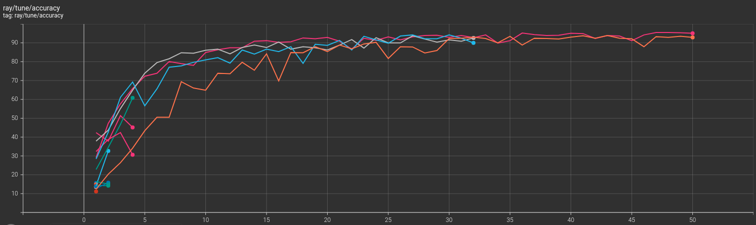
We can clearly see the searches that were terminated before 50 epochs by the scheduler.

Next Steps and Bonus Kaggle Notebook

Next, you can try your own experiments on different datasets. Maybe use the image resizing as one of the hyperparameters as well.

You may also take a look at this Kaggle Notebook. Here, after training and validation, we also carry out testing on a held-out test set. We use a Blood Cell Images dataset here which has more images compared to the one used in this tutorial. Hopefully, this will even expand your learning experience. Do let us know in the comment section of your experience with different experiments.

Summary and Conclusion

We carried out Random Hyperparameter Search and Tuning using Ray Tune and PyTorch in this tutorial. You saw how to create an entire pipeline for hyperparameter search using Ray Tune, how to use GPUs, and even visualized the proper logs of the searches. I hope that this was a good learning experience for you.

If you have any doubts, thoughts, or suggestions, please leave them in the comment section. I will surely address them.

You can contact me using the Contact section. You can also find me on LinkedIn, and Twitter.