Manual Hyperparameter Tuning in Deep Learning using PyTorch

In this post, we will carry out hyperparameter tuning for an image classification task in deep learning. But we will not use any of the tools or libraries that are already available. Instead, we will do manual hyperparameter tuning in deep learning image classification.

In the previous post, we got to know about the theoretical aspects of hyperparameter tuning in deep learning. That includes the hyperparameters related to the neural network model, the dataset, and the optimizer. If you are new to hyperparameter tuning in deep learning, then you may go through the following post first to get an insight into what all we can tune while carrying out a deep learning project.

An Introduction to Hyperparameter Tuning in Deep Learning

After going through the above post, you will also have an idea of the libraries that are available for hyperparameter tuning in deep learning.

Hyperparameter tuning in machine learning is an integral part of building a good model. Libraries like Scikit-Learn already provide good tools to do so. Then again, those are mostly applicable to the learning algorithms that we use within the Scikit-Learn environment.

In deep learning, the approach changes a bit.

Let’s now see what are all the points that we will cover in this post:

• We will begin with the exploration of the dataset that we will use.
• Then check out the directory structure for the project.
• We will write the code to carry out manual hyperaparameter tuning in deep learning using PyTorch. A few of the hyperparameters that we will control are:
  • The learning rate of the optimizer.
  • The output channels in the convolutional layers of the neural network model.
  • The output features in the fully connected layers of the neural network model.
  • Number of epochs to train for.
  • As this is an image classification task, we will also try to tune the image input size to the neural network model.
• We will end the post with an analysis which hyperparameters worked best and what might be the reason for that.

A Few Pointers to Keep in Mind

To carry out hyperparameter tuning in deep learning, we have to look at other tools dedicated to this task. Although there are many, in this post, we will do everything manually. We will write all the code to carry out manual hyperparameter tuning in deep learning. So, here are a few pointers regarding that:

• There are a lot of hyperpamaters to tune when we include the model, the dataset, and the optimizer.
• We will try to write the code in such way that we can tune as many parameters as possible.
• Still, it will not be possible to do everything that a library can do.
• We will see all the drawbacks and opportunites for improvement as well.
• As we will be doing everything manually, we need to figure out a way to properly save each hyperparameter setting, and accuracy and loss plots for each run separately. This will help us later on to look at which hyperparameter setting produced what kind of results.

I hope that you are interested to follow this tutorial through till the end. Let’s begin.

The Dataset

We will use the Natural Images from Kaggle in this post.

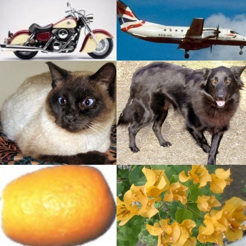
The dataset contains 6,899 images from 8 distinct classes compiled from various sources. If you want to check out the sources for each class of the dataset, please take a look at the dataset description.

The following are the classes present in the dataset:

• airplane
• car
• cat
• dog
• flower
• fruit
• motorbike
• person

Each class contains anything between 700 to 1000 images. So, it has a pretty good distribution and just the right amount of images to test different hyperparameter settings.

Be sure to download the dataset before moving further. In the next section, we will check out how to set up the input data directory along with the structure of the entire project.

The Directory Structure

Now, let’s take a look at the directory structure for this project.

├── input
│   └── natural_images
│       ├── airplane
│       ├── car
│       ├── cat
│       ├── dog
│       ├── flower
│       ├── fruit
│       ├── motorbike
│       └── person
├── outputs
│   ├── run_1
│   │   ├── accuracy.png
│   │   ├── hyperparam.yml
│   │   └── loss.png
│   ├── run_2
│   │   ├── accuracy.png
│   │   ├── hyperparam.yml
│   │   └── loss.png
│   ├── ...
└── src
    ├── datasets.py
    ├── model.py
    ├── train.py
    └── utils.py

• The input directory contains the natural_images dataset directory which in-turn contains all the class folders with the images.
• The outputs directory will contain all the plots that the training script will generate. You can see that each run’s output will be contained within it’s own folder.
• Finally we have the src directory which contains the four Python files containing all the code that we need for this post.

If you download the source code for this post, then you already have the structure in place along with the Python files. You just need to download the dataset.

PyTorch Version

PyTorch is the major requirement for this post. All the code here uses PyTorch version 1.10 (the latest at the time of writing this). If you do not have PyTorch installed in your system yet, please follow the steps here to install it.

With this, we complete all the setup we need to start the coding part for manual hyperparameter tuning in deep learning using PyTorch.

Manual Hyperparameter Tuning in Deep Learning

We know that we have four Python files. Let’s tackle the code in them in the following order:

• utils.py
• datasets.py
• model.py
• train.py

Utility and Helper Functions

We will write a few helper functions in the utils.py file. These helper functions will be to save the loss & accuracy graphs, create folders for different runs to save the outputs, and save the hyperparameter setting for each run.

The following code block contains the import statements and the first function of utils.py, that is, save_plots().

import matplotlib
import matplotlib.pyplot as plt
import os

matplotlib.style.use('ggplot')

def save_plots(
    train_acc, valid_acc, train_loss, valid_loss, 
    acc_plot_path, loss_plot_path
):
    """
    Function to save the loss and accuracy plots to disk.
    """
    # Accuracy plots.
    plt.figure(figsize=(10, 7))
    plt.plot(
        train_acc, color='green', linestyle='-', 
        label='train accuracy'
    )
    plt.plot(
        valid_acc, color='blue', linestyle='-', 
        label='validataion accuracy'
    )
    plt.xlabel('Epochs')
    plt.ylabel('Accuracy')
    plt.legend()
    plt.savefig(acc_plot_path)
    
    # Loss plots.
    plt.figure(figsize=(10, 7))
    plt.plot(
        train_loss, color='orange', linestyle='-', 
        label='train loss'
    )
    plt.plot(
        valid_loss, color='red', linestyle='-', 
        label='validataion loss'
    )
    plt.xlabel('Epochs')
    plt.ylabel('Loss')
    plt.legend()
    plt.savefig(loss_plot_path)

The save_plots() function saves the accuracy and loss plots to disk after training. It takes in the list containing training accuracy values, validation accuracy values, training loss, and validation loss values. Along with that we also provide the path for the accuracy graph and loss graph.

Next, we have the save_hyperparam() function. This function will save the hyperparameter setting for each run in a .yml file.

def save_hyperparam(text, path):
    """
    Function to save hyperparameters in a `.yml` file.

    Parameters:
    :param text: The hyperparameters dictionary.
    :param path: Path to save the hyperparmeters.
    """
    with open(path, 'w') as f:
        keys = list(text.keys())
        for key in keys:
            f.writelines(f"{key}: {text[key]}\n")

The text parameter is actually a dictionary holding all the hyperparameter settings. The path is a string indicating where to save the file.

We iterate over each key in the dictionary, extract its corresponding value and write the key-value pair in the file and save it to disk. This will actually help us later know which hyperparameter setting was used for each of the runs and we can analyze the results easily.

Finally, we have the create_run() function. Let’s check out the code first.

def create_run():
    """
    Function to create `run_<num>` folders in the `outputs` folder for each run.
    """
    num_run_dirs = len(os.listdir('../outputs'))
    run_dir = f"../outputs/run_{num_run_dirs+1}"
    os.makedirs(run_dir)
    return run_dir

The create_run() function will be called at the beginning of each training session. It will check for the number of folders inside the outputs directory. Then it will create a folder with the name run_<num> where <num> is the number of folders already present + 1. So, it will automatically create a separate folder for each run to save the graphs and hyperparameter settings.

Doing the above will actually help us differentiate each run effectively. As each of the hyperparameter .yml files will be in the same run folder, so, we can easily check the loss and accuracy graphs along with the hyperparameter settings for that specific training.

The above is all the code we need for the utils.py file.

Preparing the Dataset

This section is pretty much important. We need to prepare the image classification dataset in proper format before we can begin the training.

One thing to note here is the dataset does not contain different splits for training and validation folders in its current form. Although it has all the images in the respective class folders. Still, we need to divide the images into a training set and a validation set.

All the code here will go into the datasets.py file.

The first code block here contains all the imports that we need along with a few constants that we need to prepare the dataset.

import torch

from torch.utils.data import DataLoader, Subset
from torchvision import datasets, transforms

# Ratio of split to use for validation.
VALID_SPLIT = 0.1
# Batch size.
BATCH_SIZE = 64
# Path to data root directory.
ROOT_DIR = '../input/natural_images'

• We will use 10% of the entire dataset for validation.
• The batch size is 64.
• And we also define the path to the root data directory.

The Training and Validation Transforms

Next, let’s define the training and validation transforms.

# Training transforms
def get_train_transform(IMAGE_SIZE):
    train_transform = transforms.Compose([
        transforms.Resize((IMAGE_SIZE, IMAGE_SIZE)),
        transforms.ToTensor(),
        transforms.Normalize(
            mean=[0.5, 0.5, 0.5],
            std=[0.5, 0.5, 0.5]
        )
    ])
    return train_transform


# Validation transforms
def get_valid_transform(IMAGE_SIZE):
    valid_transform = transforms.Compose([
        transforms.Resize((IMAGE_SIZE, IMAGE_SIZE)),
        transforms.ToTensor(),
        transforms.Normalize(
            mean=[0.5, 0.5, 0.5],
            std=[0.5, 0.5, 0.5]
        )
    ])
    return valid_transform

Note that both the transform functions accept one IMAGE_SIZE argument that defines the dimension for resizing the image. It is also one of the hyperparameters that we will control later on. None of the transforms use any image augmentation techniques. This is mostly to keep things simple here. We just resize, convert the images to tensor, and normalize them.

Function to Prepare the Training and Validation Dataset

As discussed above, we do not have training and validation directories yet. This means that we need to write some manual code to split the dataset. Let’s do that first, then get down to the explanation.

# Initial entire datasets,
# same for the entire and test dataset.
def get_datasets(IMAGE_SIZE):
    dataset = datasets.ImageFolder(ROOT_DIR, transform=get_train_transform(IMAGE_SIZE))
    dataset_test = datasets.ImageFolder(ROOT_DIR, transform=get_valid_transform(IMAGE_SIZE))
    print(f"Classes: {dataset.classes}")
    dataset_size = len(dataset)
    print(f"Total number of images: {dataset_size}")

    valid_size = int(VALID_SPLIT*dataset_size)

    # Training and validation sets
    indices = torch.randperm(len(dataset)).tolist()
    dataset_train = Subset(dataset, indices[:-valid_size])
    dataset_valid = Subset(dataset_test, indices[-valid_size:])

    print(f"Total training images: {len(dataset_train)}")
    print(f"Total valid_images: {len(dataset_valid)}")
    return dataset_train, dataset_valid, dataset.classes

Going over the important points in the get_datasets() function:

• We need to pass the IMAGE_SIZE argument to this function also which the respective transform functions will use while applying the transforms when creating the dataset and dataset_test.
• Note that both dataset and dataset_test use the entire dataset. The only difference is in the transforms applied to each of them.
• After that we calculate the number of images to use for validation on line 45.
• From lines 48 to 50, we create as many indices as there are total number of images in the dataset. We subset those into the dataset_train and dataset_valid for the training and validation dataset respectively.
• Finally, we return the datasets and the class names as well.

Preparing the Data Loaders

The final part of dataset preparation is getting the data loaders ready.

# Training and validation data loaders.
def get_data_loaders(IMAGE_SIZE):
    dataset_train, dataset_valid, dataset_classes = get_datasets(IMAGE_SIZE)
    train_loader = DataLoader(
        dataset_train, batch_size=BATCH_SIZE, shuffle=True, num_workers=4
    )
    valid_loader = DataLoader(
        dataset_valid, batch_size=BATCH_SIZE, shuffle=False, num_workers=4
    )
    return train_loader, valid_loader, dataset_classes

The get_data_loaders() function also accepts the IMAGE_SIZE argument which gets passed on to the get_datasets() function. We create the train_loader and valid_loader from the respective datasets with 4 num_workers so that the preprocessing and transform steps will be much faster. After the data loader preparation we just return them along with the class names.

This function will be called from the training script by passing the IMAGE_SIZE as the argument.

With this, we complete the dataset preparation code as well.

The Neural Network Model

For this manual hyperparameter tuning in deep learning project, we will build a custom neural network. The architecture will be pretty much straightforward.

We will write the code in such a way that we will be able to control the output channels of the first 2D convolutional layer and the output features of the first fully connected layer.

Let’s write the code in model.py file.

The following code block contains the class for the entire neural network architecture.

import torch.nn as nn
import torch.nn.functional as F
import torch

class CustomNet(nn.Module):
    def __init__(self, first_conv_out, first_fc_out):
        super().__init__()

        self.first_conv_out = first_conv_out
        self.first_fc_out = first_fc_out

        # All Conv layers.
        self.conv1 = nn.Conv2d(3, self.first_conv_out, 5)
        self.conv2 = nn.Conv2d(self.first_conv_out, self.first_conv_out*2, 3)
        self.conv3 = nn.Conv2d(self.first_conv_out*2, self.first_conv_out*4, 3)
        self.conv4 = nn.Conv2d(self.first_conv_out*4, self.first_conv_out*8, 3)
        self.conv5 = nn.Conv2d(self.first_conv_out*8, self.first_conv_out*16, 3)

        # All fully connected layers.
        self.fc1 = nn.Linear(self.first_conv_out*16, self.first_fc_out)
        self.fc2 = nn.Linear(self.first_fc_out, self.first_fc_out//2)
        self.fc3 = nn.Linear(self.first_fc_out//2, 8)

        # Max pooling layers
        self.pool = nn.MaxPool2d(2, 2)

    def forward(self, x):
        x = self.pool(F.relu(self.conv1(x)))
        x = self.pool(F.relu(self.conv2(x)))
        x = self.pool(F.relu(self.conv3(x)))
        x = self.pool(F.relu(self.conv4(x)))
        x = self.pool(F.relu(self.conv5(x)))

        # Flatten 
        bs, _, _, _ = x.shape
        x = F.adaptive_avg_pool2d(x, 1).reshape(bs, -1)
        x = F.relu(self.fc1(x))
        x = F.relu(self.fc2(x))
        x = self.fc3(x)
        return x

if __name__ == '__main__':
    model = CustomNet()
    tensor = torch.randn(1, 3, 224, 224)
    output = model(tensor)
    print(output.shape)

Okay, let’s check out what is happening here.

• We initialize the __init__() method with first_conv_out and first_fc_out variables (lines 9 and 10). These two are hyperparameters that we will pass on from the training script while initializing the model. Specifically, they define the first 2D convolutional layer’s output channels and first fully connected layer’s output features. According to these two the rest of the neural network gets built.
• The subsequent 2D convolutional layer will keep on doubling the output channel size. And subsequent fully connected layers following the first one will keep on halving the output features.
• We apply 2D max-pooling to each layer along with ReLU activation.
• While flattening the features, we use adaptive_avg_pool2d() along with reshape() on line 36. This will ensure that we can give different image size as inputs to the neural network model. It is necessary as the input image size is also one of the hyperparameters that we will tune.
• We also have a if __name__ == '__main__' block just to check the output of the network if we execute the model.py file directly.

The neural network is quite simple. It is just a stacking of convolutional and fully connected layers with the ability to take in dynamic input image sizes.

The Training Script

The training script is the one we will execute to carry out all the hyperparameter experiments. It contains the:

• The training function.
• The validation function.
• The flags defining all the hyperparameters.
• The training loop.

Let’s start writing the code in train.py.

Starting with the imports.

import torch
import argparse
import torch.nn as nn
import torch.optim as optim

from tqdm.auto import tqdm

from model import CustomNet
from utils import save_hyperparam, save_plots, create_run
from datasets import get_data_loaders

Along with all the required libraries, we also import the neural network class, that is, CustomNet, the helper functions from the utils module and function to load the data loaders.

The next code block contains the training function.

# Training function.
def train(model, trainloader, optimizer, criterion):
    model.train()
    print('Training')
    train_running_loss = 0.0
    train_running_correct = 0
    counter = 0
    for i, data in tqdm(enumerate(trainloader), total=len(trainloader)):
        counter += 1
        image, labels = data
        image = image.to(device)
        labels = labels.to(device)
        optimizer.zero_grad()
        # Forward pass.
        outputs = model(image)
        # Calculate the loss.
        loss = criterion(outputs, labels)
        train_running_loss += loss.item()
        # Calculate the accuracy.
        _, preds = torch.max(outputs.data, 1)
        train_running_correct += (preds == labels).sum().item()
        # Backpropagation.
        loss.backward()
        # Update the optimizer parameters.
        optimizer.step()
    
    # Loss and accuracy for the complete epoch.
    epoch_loss = train_running_loss / counter
    epoch_acc = 100. * (train_running_correct / len(trainloader.dataset))
    return epoch_loss, epoch_acc

The train() function accepts the model, training data loader, the optimizer, and loss function (criterion) as the parameters. It is a standard PyTorch image classification training function that iterates through the batches of images. Then feeds them to the neural network model, gets the outputs, calculates the loss, backpropagates the gradients, and updates the optimizer.

In the end, we return the loss and accuracy for each epoch.

Now, the validation function.

# Validation function.
def validate(model, testloader, criterion, class_names):
    model.eval()
    print('Validation')
    valid_running_loss = 0.0
    valid_running_correct = 0
    counter = 0
    
    with torch.no_grad():
        for i, data in tqdm(enumerate(testloader), total=len(testloader)):
            counter += 1
            
            image, labels = data
            image = image.to(device)
            labels = labels.to(device)
            # Forward pass.
            outputs = model(image)
            # Calculate the loss.
            loss = criterion(outputs, labels)
            valid_running_loss += loss.item()
            # Calculate the accuracy.
            _, preds = torch.max(outputs.data, 1)
            valid_running_correct += (preds == labels).sum().item()
        
    # Loss and accuracy for the complete epoch.
    epoch_loss = valid_running_loss / counter
    epoch_acc = 100. * (valid_running_correct / len(testloader.dataset))
    return epoch_loss, epoch_acc

The validation function is almost similar to the training function. Except we do not need to backpropagate the gradients or update the optimizer.

We still return the loss and accuracy values for each epoch.

The Main Code Block

Now coming to the main code block. Here, we will create the directory for each run to save the outputs and hyperparameter settings. We will also initialize all the hyperparameters and write the training loop.

The next block contains the entire main code.

if __name__ == '__main__':
    # Create the current running directory to save plots and hyperparameters.
    run_dir = create_run()

    # Construct the argument parser.
    parser = argparse.ArgumentParser()
    parser.add_argument('-e', '--epochs', type=int, default=20,
        help='number of epochs to train our network for')
    parser.add_argument(
        '-lr', '--learning-rate', dest='learning_rate', default=0.01, 
        type=float, help='learning rate for the optimizer'
    )
    parser.add_argument(
        '-co', '--conv-out', dest='conv_out', default=8, type=int,
        help='output channels for first convolutional layers'
    )
    parser.add_argument(
        '-fo', '--fc-out', dest='fc_out', default=256, type=int,
        help='output units for first fully-connected layer' 
    )
    parser.add_argument(
        '-s', '--image-size', dest='image_size', default=224, type=int,
        help='size to resize image to'
    )
    args = vars(parser.parse_args())
    
    # Write the hyperparameters to a YAML file.
    save_hyperparam(args, f"../outputs/{run_dir}/hyperparam.yml")


    # Learning parameters. 
    lr = args['learning_rate']
    epochs = args['epochs']
    device = ('cuda' if torch.cuda.is_available() else 'cpu')
    print(f"Computation device: {device}\n")

    # Build the model.
    model = CustomNet(args['conv_out'], args['fc_out']).to(device)
    print(model)
    # Total parameters and trainable parameters.
    total_params = sum(p.numel() for p in model.parameters())
    print(f"{total_params:,} total parameters.")
    total_trainable_params = sum(
        p.numel() for p in model.parameters() if p.requires_grad)
    print(f"{total_trainable_params:,} training parameters.\n")

    # Optimizer.
    optimizer = optim.Adam(model.parameters(), lr=lr)
    # Loss function.
    criterion = nn.CrossEntropyLoss()

    # Get the training and validation data loaders.
    train_loader, valid_loader, dataset_classes = get_data_loaders(
        args['image_size']
    )

    # Lists to keep track of losses and accuracies.
    train_loss, valid_loss = [], []
    train_acc, valid_acc = [], []
    # Start the training.
    for epoch in range(epochs):
        print(f"[INFO]: Epoch {epoch+1} of {epochs}")
        train_epoch_loss, train_epoch_acc = train(model, train_loader, 
                                                optimizer, criterion)
        valid_epoch_loss, valid_epoch_acc = validate(model, valid_loader,  
                                                    criterion, dataset_classes)
        train_loss.append(train_epoch_loss)
        valid_loss.append(valid_epoch_loss)
        train_acc.append(train_epoch_acc)
        valid_acc.append(valid_epoch_acc)
        print(f"Training loss: {train_epoch_loss:.3f}, training acc: {train_epoch_acc:.3f}")
        print(f"Validation loss: {valid_epoch_loss:.3f}, validation acc: {valid_epoch_acc:.3f}")
        print('-'*50)

    # Save the loss and accuracy plots.
    save_plots(
        train_acc, valid_acc, train_loss, valid_loss, 
        f"../outputs/{run_dir}/accuracy.png",
        f"../outputs/{run_dir}/loss.png"
    )
    print('TRAINING COMPLETE')

• On line 71, we create the run_<num> directory for the current run. This will be run_1, run_2, and so on.
• Starting from line 73, we construct the argument parser and define the flags for all the hyperparameters we want to tune. These include:
  • The number of epochs.
  • The learning rate.
  • The output channels for the first convolutional layer of the neural network.
  • The output features for the first fully connected layer of the neural network.
  • And the input image size.

All of the above have a default value as well.

• On line 96, we call the save_hyperparam() function to save the hyperparameters for the current run in the .yml file.
• Then we define the learning parameters like the learning rate and the number of epochs along with the computation device.
• After building the model, initializing the optimizer, and loading the data loaders, we start the training loop.
• After each epoch, we print the current loss and accuracy.
• At the end, we save the loss and accuracy graphs to disk.

With this, we complete all the code that we need. The only thing left now is to execute the training script with different hyperparameters and check out the results.

Training with Different Hyperparameter Settings

We will carry a total of 6 manual hyperparameter tuning deep learning experiments here. Each training will create a new run folder in the outputs directory.

To start the experiments, open your command line/terminal in the src directory.

Run 1

For the first run, we will use the default hyperparameters. Execute the following to start the training.

python train.py --epochs 20 --learning-rate 0.01 --conv-out 8 --fc-out 256 --image-size 224

The following is the shortened output.

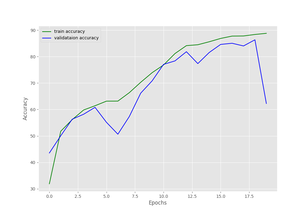
Computation device: cuda

CustomNet(
  (conv1): Conv2d(3, 8, kernel_size=(5, 5), stride=(1, 1))
  (conv2): Conv2d(8, 16, kernel_size=(3, 3), stride=(1, 1))
  (conv3): Conv2d(16, 32, kernel_size=(3, 3), stride=(1, 1))
  (conv4): Conv2d(32, 64, kernel_size=(3, 3), stride=(1, 1))
  (conv5): Conv2d(64, 128, kernel_size=(3, 3), stride=(1, 1))
  (fc1): Linear(in_features=128, out_features=256, bias=True)
  (fc2): Linear(in_features=256, out_features=128, bias=True)
  (fc3): Linear(in_features=128, out_features=8, bias=True)
  (pool): MaxPool2d(kernel_size=2, stride=2, padding=0, dilation=1, ceil_mode=False)
)
165,720 total parameters.
165,720 training parameters.

Classes: ['airplane', 'car', 'cat', 'dog', 'flower', 'fruit', 'motorbike', 'person']
Total number of images: 6899
Total training images: 6210
Total valid_images: 689
[INFO]: Epoch 1 of 20
Training
100%|████████████████████████████████████████████████████████████████████| 98/98 [00:03<00:00, 27.90it/s]
Validation
100%|████████████████████████████████████████████████████████████████████| 11/11 [00:00<00:00, 22.56it/s]
Training loss: 1.923, training acc: 22.754
Validation loss: 1.794, validation acc: 28.302
--------------------------------------------------
...
[INFO]: Epoch 20 of 20
Training
100%|████████████████████████████████████████████████████████████████████| 98/98 [00:03<00:00, 30.61it/s]
Validation
100%|████████████████████████████████████████████████████████████████████| 11/11 [00:00<00:00, 21.97it/s]
Training loss: 0.350, training acc: 86.296
Validation loss: 0.376, validation acc: 85.341
--------------------------------------------------
TRAINING COMPLETE

We can see that with the default hyperparameter settings, we end up with a validation accuracy of 85.341% and validation loss o 0.376.

Let’s check out the loss and accuracy graphs.

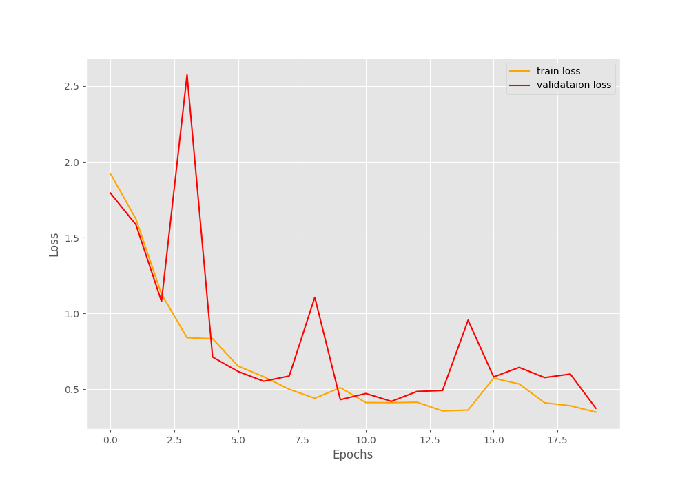
As of now, we do not have anything to compare the current results with. Although it seems like a bit more training would have helped.

Run 2

This time we will change the learning rate to 0.001. Also, from here onward, we will just check out the last epoch’s result from the output block for the sake of brevity.

python train.py --epochs 20 --learning-rate 0.001 --conv-out 8 --fc-out 256 --image-size 224

[INFO]: Epoch 20 of 20
Training
100%|████████████████████████████████████████████████████████████████████| 98/98 [00:03<00:00, 31.04it/s]
Validation
100%|████████████████████████████████████████████████████████████████████| 11/11 [00:00<00:00, 21.61it/s]
Training loss: 0.279, training acc: 88.808
Validation loss: 1.339, validation acc: 62.264
--------------------------------------------------
TRAINING COMPLETE

The training results seem to be better this time but the validation results are quite worse.

It seems like the validation results are worse particularly in the last epoch. As we are not using any seed value for reproducibility here, it might also be a one-off thing, and running the experiment again might give better results. But that is not a lasting solution.

Run 3

Let’s double the number of output channels and output features for the convolutional layer and fully connected layer respectively. This will result in a larger model with more parameters.

python train.py --epochs 20 --learning-rate 0.01 --conv-out 16 --fc-out 512 --image-size 224

[INFO]: Epoch 20 of 20
Training
100%|████████████████████████████████████████████████████████████████████| 98/98 [00:03<00:00, 27.77it/s]
Validation
100%|████████████████████████████████████████████████████████████████████| 11/11 [00:00<00:00, 22.17it/s]
Training loss: 2.073, training acc: 14.171
Validation loss: 2.065, validation acc: 14.804
--------------------------------------------------
TRAINING COMPLETE

It seems like the neural network model did not learn at all.

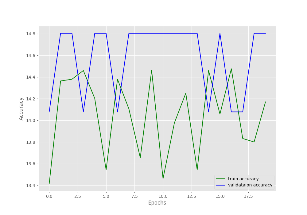
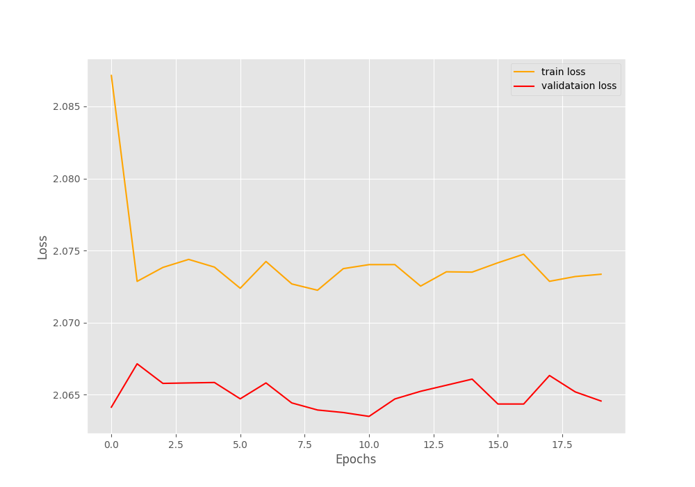
From the plots, it is pretty clear that these hyperparameters are not at all optimal. Training for any number of epochs will not give relevant results.

Run 4

This time we keep those above settings for the convolutional and fully connected layers. And change the learning rate to 0.001.

python train.py --epochs 20 --learning-rate 0.001 --conv-out 16 --fc-out 512 --image-size 224

[INFO]: Epoch 20 of 20
Training
100%|████████████████████████████████████████████████████████████████████| 98/98 [00:03<00:00, 29.15it/s]
Validation
100%|████████████████████████████████████████████████████████████████████| 11/11 [00:00<00:00, 21.37it/s]
Training loss: 0.200, training acc: 91.997
Validation loss: 0.327, validation acc: 88.679
--------------------------------------------------
TRAINING COMPLETE

This looks pretty good. Let’s check out the graphs.

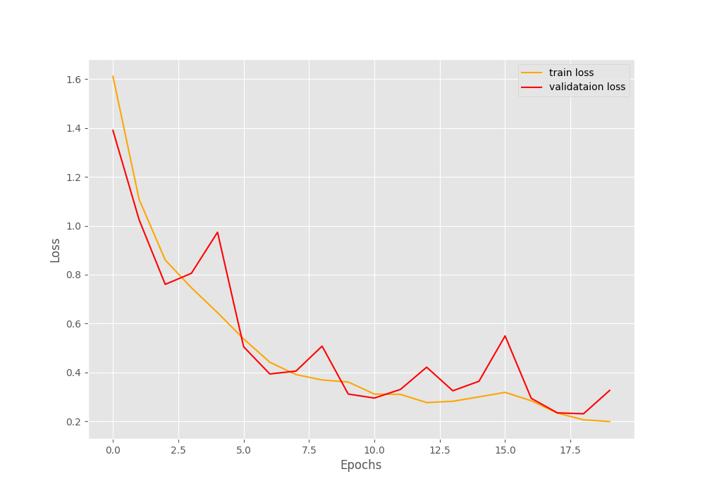
From the graphs also, it is pretty clear that these settings give the best result till now. Although the loss plot indicates a bit of overfitting by the end of 20 epochs. Training any longer might actually worsen the results.

Run 5

Now, along with the previous settings, increasing the number of epochs to 35.

python train.py --epochs 35 --learning-rate 0.001 --conv-out 16 --fc-out 512 --image-size 224

[INFO]: Epoch 35 of 35
Training
100%|████████████████████████████████████████████████████████████████████| 98/98 [00:03<00:00, 28.00it/s]
Validation
100%|████████████████████████████████████████████████████████████████████| 11/11 [00:00<00:00, 21.17it/s]
Training loss: 0.110, training acc: 96.216
Validation loss: 0.265, validation acc: 93.469
--------------------------------------------------
TRAINING COMPLETE

The validation numbers seem to have improved.

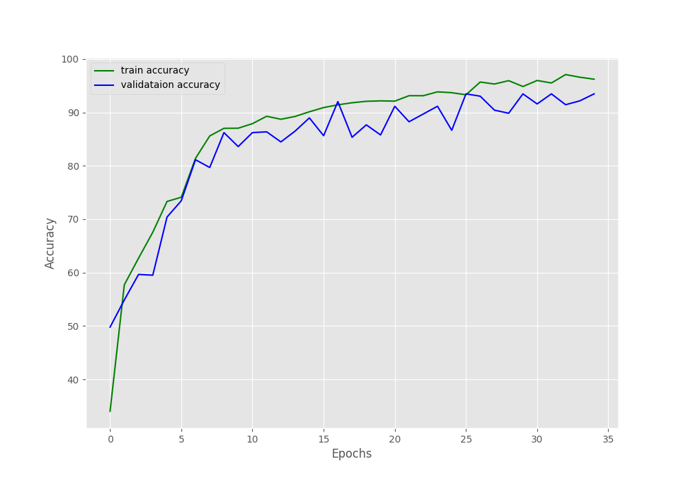
The validation accuracy seems to be improving. But from the validation loss plot, we can clearly see signs of overfitting after 35 epochs.

Run 6

This is the final run. We will keep the above settings. And trying to avoid overfitting, let’s give the neural network model a bit more information to look at. That is increase the image size to 320×320. Also, increase the number of epochs to 50.

python train.py --epochs 50 --learning-rate 0.001 --conv-out 16 --fc-out 512 --image-size 320

[INFO]: Epoch 50 of 50
Training
100%|████████████████████████████████████████████████████████████████████| 98/98 [00:06<00:00, 14.20it/s]
Validation
100%|████████████████████████████████████████████████████████████████████| 11/11 [00:00<00:00, 13.50it/s]
Training loss: 0.090, training acc: 96.473
Validation loss: 0.203, validation acc: 93.179
--------------------------------------------------
TRAINING COMPLETE

The above validation results look good, in fact, seem like the best till now.

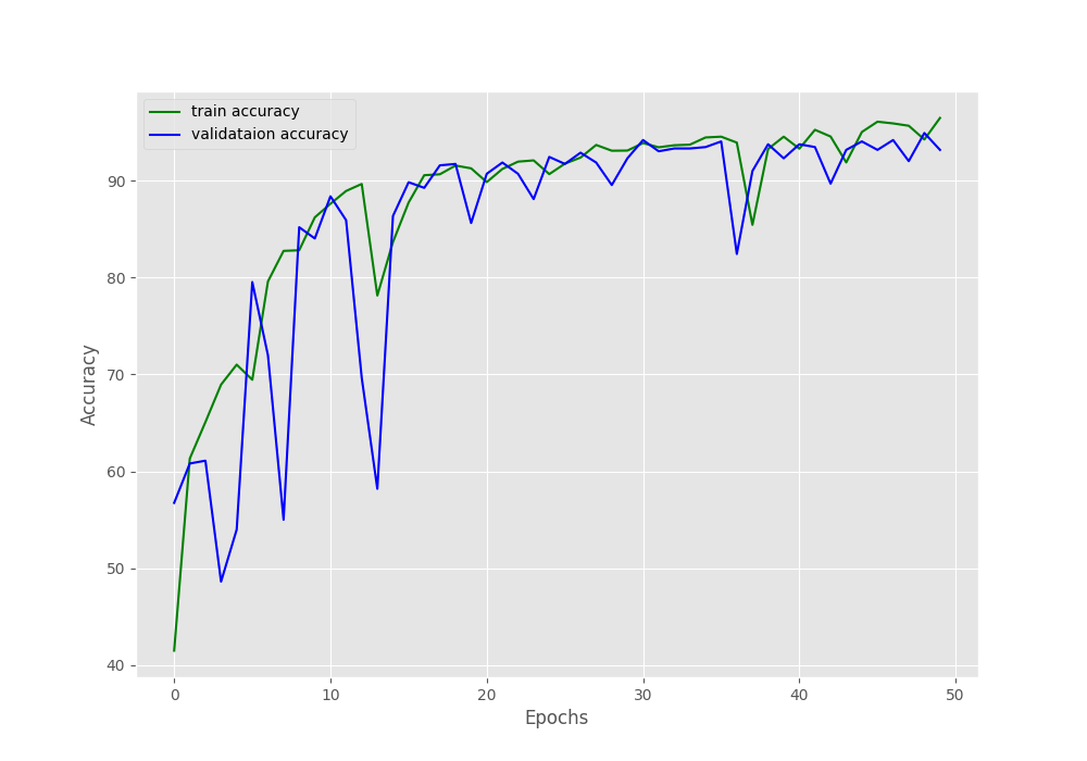
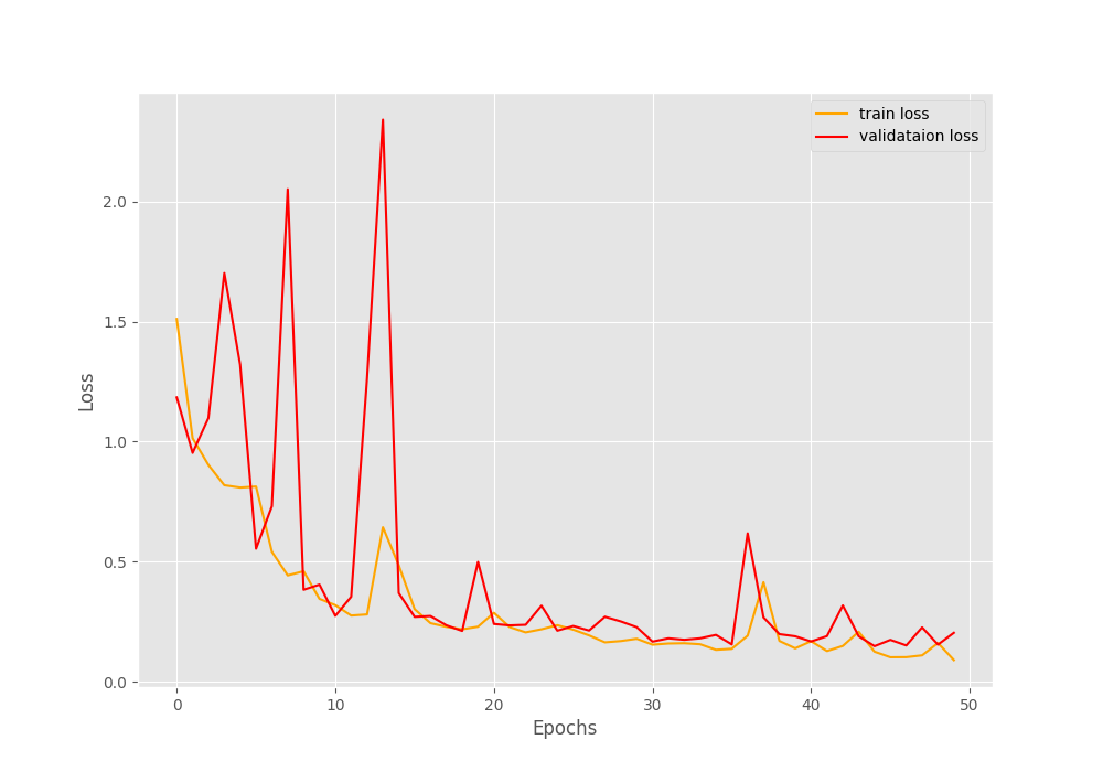
From the graphs, we can see that increasing the image resolution does the trick. Although a bit of fluctuation is present in the initial epochs, by the end of training we have the least validation loss as of yet.

Takeaway

From the above experiments, we come to know that we need to deal with a lot of hyperparameters to find the best settings to get the best results.

And with the increase in the number of hyperparameters, the task will become even more difficult. In fact, we could feel that changing each hyperparameter manually was not the best way to deal with the issue. Also, we have not used the batch size as one of the hyperparameters in the above experiments. Yet, we had so many variables to deal with.

The above experiments clearly show how cumbersome manual hyperparameter tuning in deep learning can be. That’s why we have so many tools and libraries that we discussed in the previous post. In future posts, we will start to explore one of them for hyperparameter tuning and eventually move on to others. It is also worth noting that manual hyperparameter tuning is one of the least effective ways to find the optimal setting if you are not an experienced deep learning practitioner or researcher.

Summary and Conclusion

In this tutorial, we wrote the code to carry out manual hyperparameter tuning in deep learning. We saw what are some of the obvious hyperparameters that we can tune easily. Along with that we also ran experiments with different settings and discussed the drawbacks of manual hyperparameter tuning. I hope that this tutorial was helpful to you.

If you have any doubts, thoughts, or suggestions, please leave them in the comment section. I will surely address them.

You can contact me using the Contact section. You can also find me on LinkedIn, and Twitter.