PlantVillage Dataset Disease Recognition using PyTorch

The first step to good agricultural yield is protecting the plants from diseases. Early plant disease recognition and prevention is the first step in this regard. But manual disease recognition is time-consuming and costly. This is one of those use cases, where deep learning can be used proactively for great benefit. Using deep learning, we can recognize plant diseases very effectively. Large scale plant disease recognition using deep learning can cut costs to a good extent. In this blog post, we will use deep learning for disease recognition on the PlantVillage dataset using deep learning and PyTorch.

This blog post is the first one in a series of three blog posts. We will start with the PlantVillage dataset disease recognition. Then we will move on to PlantDoc dataset for plant disease recognition using deep learning. Finally, we will apply deep learning based object detection for large scale disease detection and localization.

I hope that this series becomes worthwhile and useful to make the use of deep learning for plant pathology slightly easier.

What Will We Cover in This Blog Post

This blog post is like a mini deep learning project. Here, we will train three deep convolutional neural network models. They are:

• MobileNet V3
• ShuffleNet V2
• EfficientNetB0

We are choosing smaller neural network models so that we can iterate faster through the experiments. This also gives us a chance to check whether smaller (mobile based) classification models are suitable for complex problems or not.

After training, we will run all three trained models on a held-out test out. Then we will choose the best-performing model for inference on some real-life unseen images.

This project on PlantVillage dataset for disease recognition will act as a stepping stone for the next two blog posts.

We will cover the following topics in this blog post:

• We will start with a detailed exploration of the PlantVillage dataset.
• Then we will move on to directory structuring and planning.
• As the codebase for this project is quite large, we will not discuss each Python file. We will only discuss the important parts. All the code files will be available for download.
• Next, we will move on to training and testing an image recognition neural network.
  • We will fine tune pretrained MobileNet V3, ShuffleNet V2, and EfficientNetB0 models in this section.
• After that, we will also run inference on some real-life plant disease images collected from the internet.
• Finally, we will discuss the benefits, drawbacks, and future possibilities of the project.

Let’s jump into this exciting project.

Exploring the Plant Village Dataset

For this blog post, we will use the PlantVillage dataset from Kaggle.

The PlantVillage dataset contains more than 50000 images of healthy and infected leaves. All the images have been collected via the PlantVillage online platform.

All the images were captured in controlled settings with a static background.

The dataset contains 38 classes. Each class belongs to a different plant or crop and may resemble a particular disease from a particular plant. For example, the dataset contains multiple diseases from the Apple plant. They are Apple_Scab, Black_rot, and Cedar_apple_rust.

Each class has a different directory.

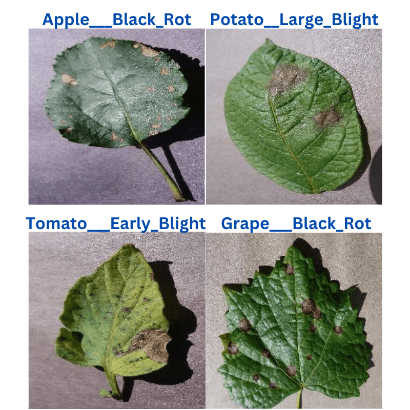
For now, let’s take a look at some of the images from the dataset.

The following block shows the directory structure after downloading and extracting the dataset.

├── color
│   ├── Apple___Apple_scab
│   ├── Apple___Black_rot
│   ...
│   └── Tomato___Tomato_Yellow_Leaf_Curl_Virus
├── grayscale
│   ├── Apple___Apple_scab
│   ├── Apple___Black_rot
│   ...
│   └── Tomato___Tomato_Yellow_Leaf_Curl_Virus
└── segmented
    ├── Apple___Apple_scab
    ├── Apple___Black_rot
    ...
    └── Tomato___Tomato_Yellow_Leaf_Curl_Virus

The dataset contains three different directories, each with the same class names.

• In the color directory, we have all the RGB images in each of the class folders. This is the folder we will use for image classification.
• The grayscale directory contains the images but in single channel grayscale format.
• Finally, the segmented directory contains the same images in the same structure with only the segmented leaf.

As we will be using the images from the color directory in this dataset, we can ignore the other two.

For now, you may go ahead and download the dataset from here. In the next section, we will see how to structure the project after extracting the dataset.

Directory Structure

The following block shows the directory structure of the entire project.

.
├── input
│   ├── inference_data
│   ├── plantvillage dataset
│   │   ├── color
│   │   ├── grayscale
│   │   └── segmented
│   └── test
│       ├── Apple___Apple_scab
│       ...
│       └── Tomato___Tomato_Yellow_Leaf_Curl_Virus
├── outputs
│   ├── test_results
│   │   ├── test_image_1000.png
│   │   ...
│   │   └── test_image_9.png
│   ├── accuracy.png
│   ├── best_model.pth
│   ├── loss.png
│   └── model.pth
└── src
    ├── class_names.py
    ├── datasets.py
    ├── inference.py
    ├── model.py
    ├── prepare_test_data.py
    ├── test.py
    ├── train.py
    └── utils.py

• The dataset resides in the input directory. Along with the plantvillage dataset (that we saw in the previous section), we also have inference_data and test directories. The former contains a few images from the internet to be used for inference after training. And the latter is a small subset of the original dataset to be used for testing. Later on, we will go through the process of creating the test set.
• The outputs directory contains all the outputs from training, testing, and inference.
• There are 8 scripts in the src directory. We will discuss the necessary details of each Python file in their respective section.

Go ahead and download the zip file for this project. All the code files are provided. You only need to arrange the dataset in the above structure after downloading it from here.

PyTorch Version

The code for this blog needs at least PyTorch version 1.12.0.

You can install/upgrade PyTorch from the official website here.

There are other common dependencies like OpenCV which you may install as you proceed with training, testing, and inference.

PlantVillage Disease Recognition using PyTorch

Let’s get into the details of the training section now. We will discuss all the essential details that we need to train a deep learning model for PlantVillage dataset disease recognition using PyTorch.

All the Python files reside inside the src directory.

Download Code

The Class Names

The PlantVillage dataset contains 38 classes. For this reason, tt is better to create a list and save them in a separate Python file which we can import anywhere we want.

In this project, we keep them in the class_names.py file.

class_names = [
    "Apple___Apple_scab",
    "Apple___Black_rot",
    "Apple___Cedar_apple_rust",
    "Apple___healthy",
    "Blueberry___healthy",
    "Cherry_(including_sour)___Powdery_mildew",
    "Cherry_(including_sour)___healthy",
    "Corn_(maize)___Cercospora_leaf_spot Gray_leaf_spot",
    "Corn_(maize)___Common_rust_",
    "Corn_(maize)___Northern_Leaf_Blight",
    "Corn_(maize)___healthy",
    "Grape___Black_rot",
    "Grape___Esca_(Black_Measles)",
    "Grape___Leaf_blight_(Isariopsis_Leaf_Spot)",
    "Grape___healthy",
    "Orange___Haunglongbing_(Citrus_greening)",
    "Peach___Bacterial_spot",
    "Peach___healthy",
    "Pepper,_bell___Bacterial_spot",
    "Pepper,_bell___healthy",
    "Potato___Early_blight",
    "Potato___Late_blight",
    "Potato___healthy",
    "Raspberry___healthy",
    "Soybean___healthy",
    "Squash___Powdery_mildew",
    "Strawberry___Leaf_scorch",
    "Strawberry___healthy",
    "Tomato___Bacterial_spot",
    "Tomato___Early_blight",
    "Tomato___Late_blight",
    "Tomato___Leaf_Mold",
    "Tomato___Septoria_leaf_spot",
    "Tomato___Spider_mites Two-spotted_spider_mite",
    "Tomato___Target_Spot",
    "Tomato___Tomato_Yellow_Leaf_Curl_Virus",
    "Tomato___Tomato_mosaic_virus",
    "Tomato___healthy"
]

There are a few points to note here:

• All the class names have two parts which are separated by three underscores (___).
• The first part contains the names of the plant, e.g. Apple or Cherry or Potato. The second part indicates either the disease name or if the plant is healthy.

Getting to know the class names a bit better helps a lot.

Prepare the Test Set

Right now, all the images are present inside their class folders without any split. We will create a test split manually and separate out 100 images from each class.

The prepare_test_data.py file contains the code for this. Further, to make the results reproducible, we also set a seed in the script. This will ensure on a particular machine, we will get the same test split every time.

You can execute it using the following command.

python prepare_test_data.py

Executing the script will give output similar to the following.

Initial number of images for class Apple___Apple_scab: 630
Final number of images for class Apple___Apple_scab: 530

Initial number of images for class Apple___Black_rot: 621
Final number of images for class Apple___Black_rot: 521
.
.
.
Initial number of images for class Tomato___Tomato_mosaic_virus: 373
Final number of images for class Tomato___Tomato_mosaic_virus: 273

Initial number of images for class Tomato___healthy: 1591
Final number of images for class Tomato___healthy: 1491

Now, we have a total of 3800 test images inside input/test directory.

The Dataset and Data Loader Preparation

The next step is to prepare the datasets and the data loaders. All the code for this is in the datasets.py file.

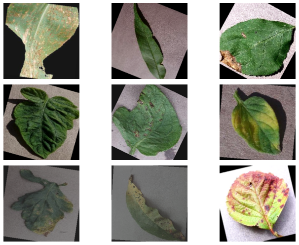
We use quite a few augmentation techniques to make sure that the model sees enough variation of the healthy and diseased leaves. They are:

• RandomHorizontalFlip
• RandomVerticalFlip
• RandomRotation
• ColorJitter
• GaussianBlur
• RandomAdjustSharpness

The figure below shows how the images look when the augmentations are applied randomly.

Apart from that, we use the following hyperparameters for the dataset preparation.

• Image size of 224×224 – resized using torchvision.transforms
• Batch size of 32
• The number of parallel workers is 4 – for multi-processing
• The validation split is 15%

It is important to keep all the above hyperparameters in mind as GPU compute timing is an integral part of any deep learning project. And as we are running multiple experiments, these hyperparameters become even more important.

Helper Scripts

We need a few simple yet important helper scripts during the training of the models on the PlantVillage dataset for disease recognition.

The utils.py file contains the code for this. These include:

• The SaveBestModel class: It will save the model to the disk whenever the current validation loss is lower compared to the previous least loss value.
• save_model function: It saves the model one final time at the end of the training.
• save_plots function: This function saves the accuracy and loss graphs at the end of training.

You may take a look at the utils.py file if you wish to know about these in detail.

The Deep Learning Models

As discussed earlier, for the PlantVillage dataset for disease recognition, we will train three models. But changing the model loading code every time we want to train a new model is a bad idea. So, we will have to figure out a way to optimize this.

Let’s take a look at the entire model.py file to get a better idea.

from torchvision import models

def model_config(model_name='mobilenetv3_large'):
    model = {
        'mobilenetv3_large': models.mobilenet_v3_large(weights='DEFAULT'),
        'shufflenetv2_x1_5': models.shufflenet_v2_x1_5(weights='DEFAULT'),
        'efficientnetb0': models.efficientnet_b0(weights='DEFAULT')
    }
    return model[model_name]

def build_model(model_name='mobilenetv3_large', fine_tune=True, num_classes=10):
    model = model_config(model_name)
    if fine_tune:
        print('[INFO]: Fine-tuning all layers...')
        for params in model.parameters():
            params.requires_grad = True
    elif not fine_tune:
        print('[INFO]: Freezing hidden layers...')
        for params in model.parameters():
            params.requires_grad = False
    if model_name == 'mobilenetv3_large':
        model.classifier[3].out_features = num_classes
    if model_name == 'shufflenetv2_x1_5':
        model.fc.out_features = num_classes
    if model_name == 'mobilenetv3_large':
        model.classifier[1].out_features = num_classes
    return model

We have two functions here:

• model_config function: This contains the model dictionary with the callable PyTorch models as values. The keys are model name strings that we will pass to the training script through the command line. We are using the default ImageNet pretrained weights for every model.
• build_model function: This function loads the pretrained model by calling the model_config function. Also, we have a few if statements to manage the number of classes in the final classification head.

That’s all we need to load the models.

The Training Script

The train.py script is the driver script for all the training experiments. Let’s cover the important bits of the file.

It contains three arguments for the command line flag:

• --epochs: To pass the number of epochs to train for.
• --learning-rate: The learning that we want to use for the optimizer. It is 0.001 by default.
• --model: This accepts a model name string. We can pass either mobilenetv3_large or shufflenetv2_x1_5 or efficientnetb0.

A few other important points about the training process:

• We will always fine tune all the layers of the model in these transfer learning experiments.
• The optimizer is SGD (Stochastic Gradient Descent) with a default learning rate of 0.001.
• As it is a multi-class problem, we are using the Cross-Entropy loss function.
• The training script saves the best model according to the least validation loss.

Till now, we have covered everything that we need to start the training process. Now, let’s jump into the training of the three models now.

Execute train.py for Training on the PlantVillage Dataset for Disease Recognition

We need to carry out three training experiments for the three models. We will train each model for 10 epochs.

All the training, testing, and inference experiments were carried out on a laptop with:

• 8th generation i7 Intel CPU
• 6GB GTX 1060 GPU
• 16GB DDR RAM

Train the MobileNet V3 Large Model

We will start with training the MobileNet V3 Large model.

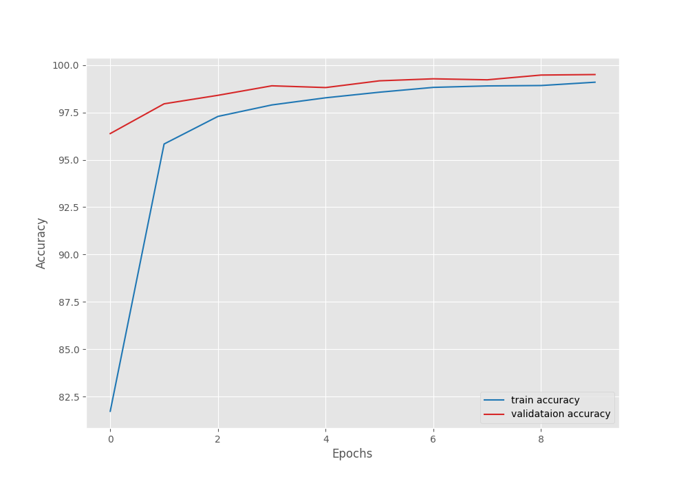
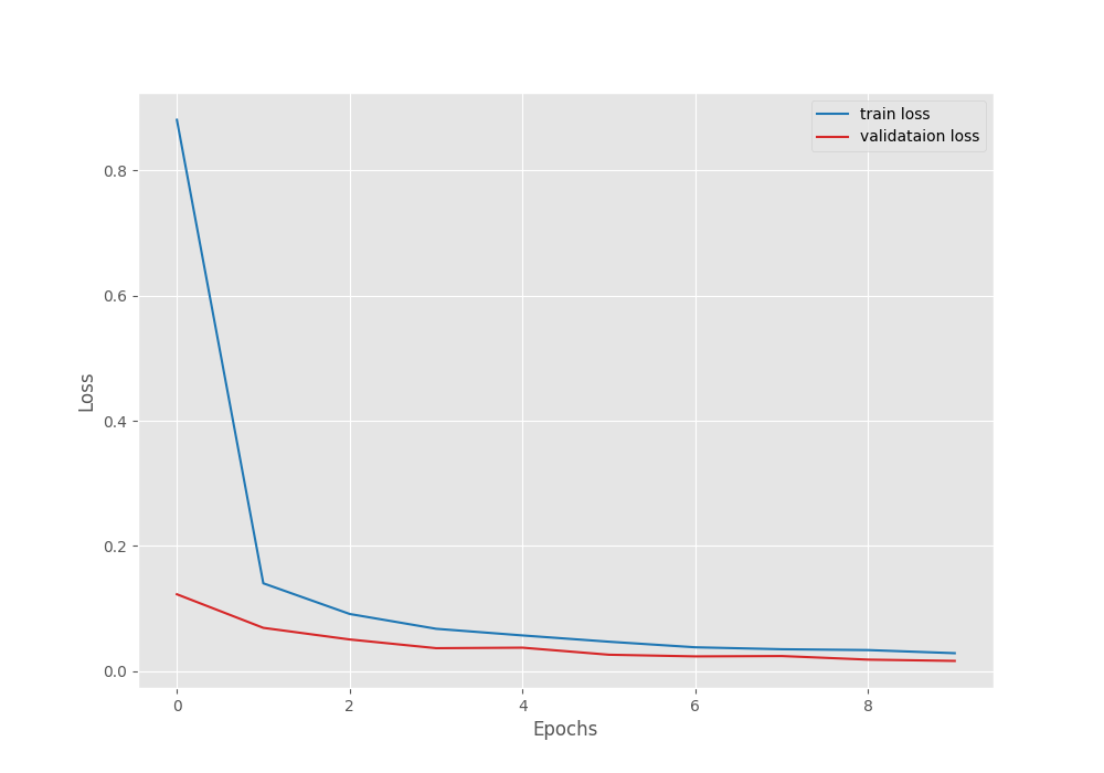
python train.py --model mobilenetv3_large --epochs 10

After the last epoch, the validation loss was 0.020, and the validation accuracy was 99.551 %.

The following are the accuracy and loss graphs.

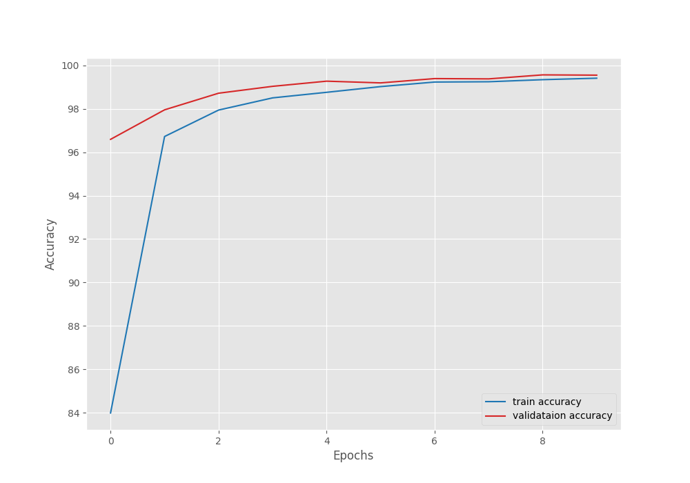
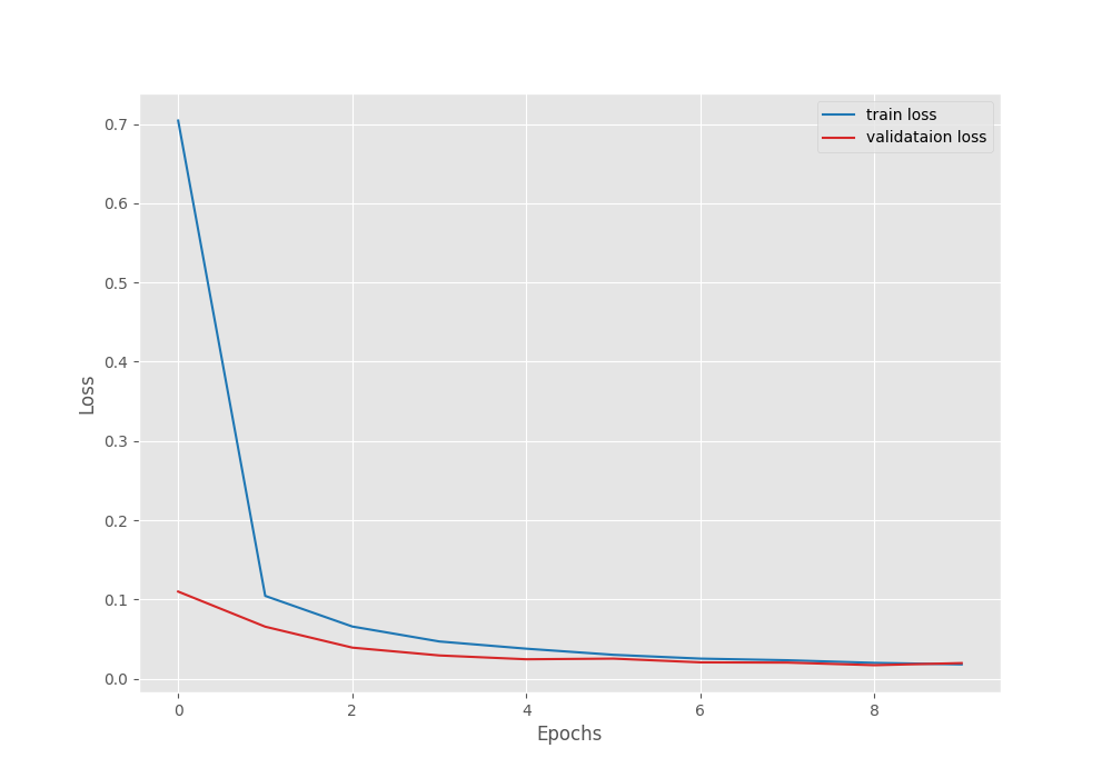
We can see that the highest accuracy and the least loss correspond to epoch 8. In fact, that is where the best model is saved as well.

Train the ShuffleNet V2 X1.5 Model

We can execute the following command to train the ShuffleNet V2 X1.5 model.

python train.py --model shufflenetv2_x1_5 --epochs 10

Here, the final epoch’s validation loss was 0.032. And the validation accuracy was 99.010. As the least loss value was after epoch 10, the last model is the best model in this case.

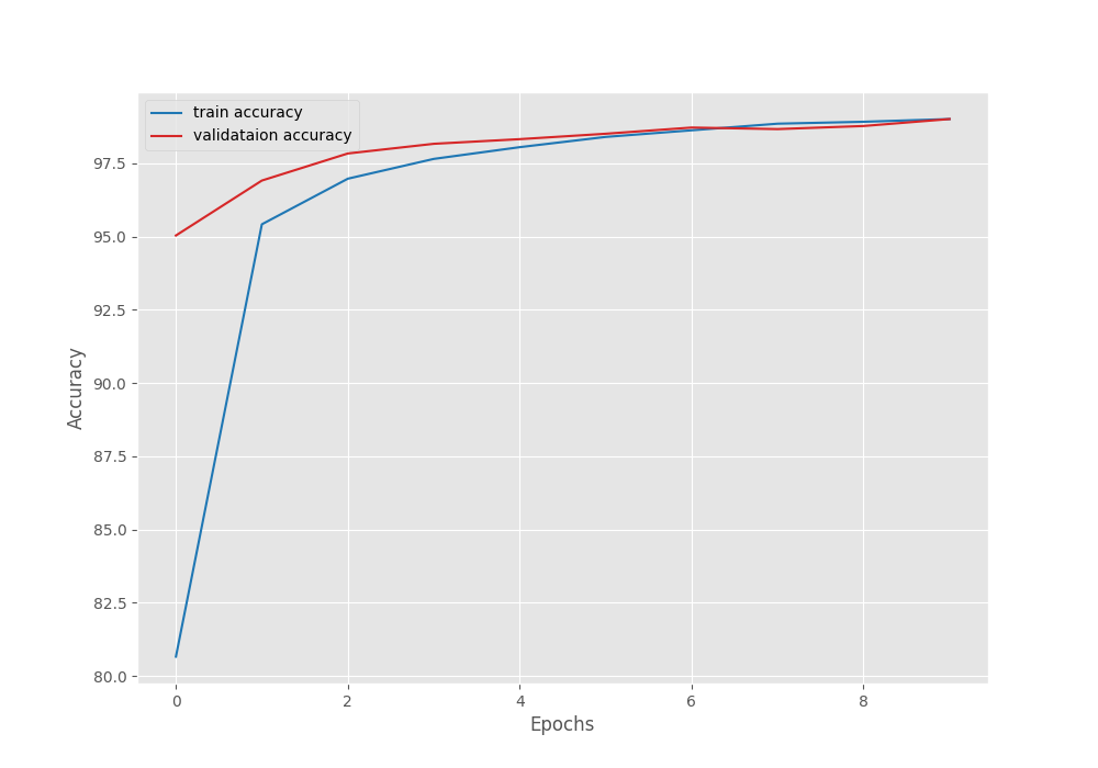
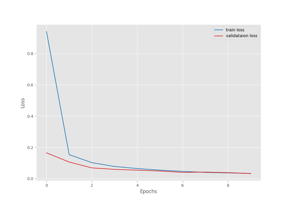
It is clear from the above graphs also that the model can learn more if we train for more epochs.

Train the EfficientNetB0 Model

This is the final training experiment.

python train.py --model efficientnetb0 --epochs 10

The best model for EfficientNetB0 on the PlantVillage disease recognition dataset was saved after epoch 10. The validation loss was 0.016 and the validation accuracy was 99.498%.

Although very close to MobileNet V3 Large model, still slightly lower in terms of validation accuracy. But note that the validation loss is also lower. So, it will all boil down to the best test accuracy which we will check in the next section.

Testing the Models

Here, we will test all the best model weights on the test dataset using the test.py script. The test.py script has a --weights flag that we can use to pass the model weights path while executing it. After that, whichever model will have the highest test accuracy, we will use that for running inference on some images from the internet.

The following are the test script execution command along with the accuracy outputs that we get for all three saved weights.

python test.py --weights ../outputs/mobilenetv3_large/best_model.pth
mobilenetv3_large
[INFO]: Freezing hidden layers...
Testing model
100%|██████████████████████████████████████████████████████████████| 3800/3800 [01:44<00:00, 36.51it/s]
Test accuracy: 99.132%

python test.py --weights ../outputs/shufflenetv2_x1_5/best_model.pth
shufflenetv2_x1_5
[INFO]: Freezing hidden layers...
Testing model
100%|██████████████████████████████████████████████████████████████| 3800/3800 [01:31<00:00, 41.44it/s]
Test accuracy: 98.711%

python test.py --weights ../outputs/efficientnetb0/best_model.pth
efficientnetb0
[INFO]: Freezing hidden layers...
Testing model
100%|██████████████████████████████████████████████████████████████| 3800/3800 [01:35<00:00, 39.85it/s]
Test accuracy: 99.289%

The following is a bar graph showing the test accuracy values of all three models.

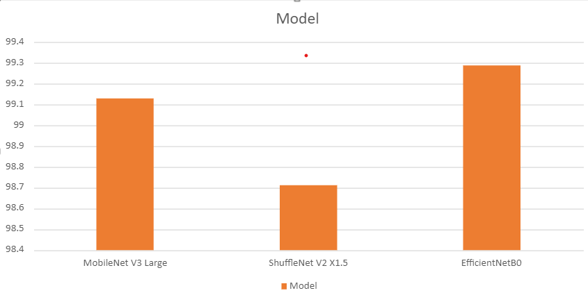
Interestingly, although EfficientNetB0 had lower best validation accuracy compared to MobileNet V3 Large, it is doing better on the test set.

Let’s use the EfficientNetB0 weights and run inference on some real-life images.

Inference for PlantVillage Dataset for Disease Recognition

For the inference, we choose three random images from the internet. They are leaves affected with:

• Apple scab
• Corn common rust
• Grape black rot
• Tomato early blight

Running inference.py script with the following command will use the best EfficientNetB0 weights for inference.

python inference.py --weights ../outputs/efficientnetb0/best_model.pth

The results will be saved to outputs/inference_results/efficientnetb0. Further, all the images are annotated with the predictions. Also, we can easily know the ground truth from the image file name.

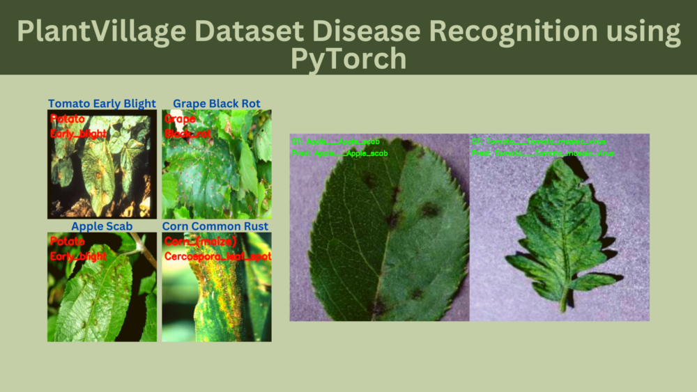
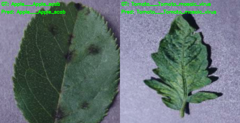
The following figure shows the inference results. The annotations on the images show the predictions which were done using the inference script. The blue text on top of each image shows the ground truth.

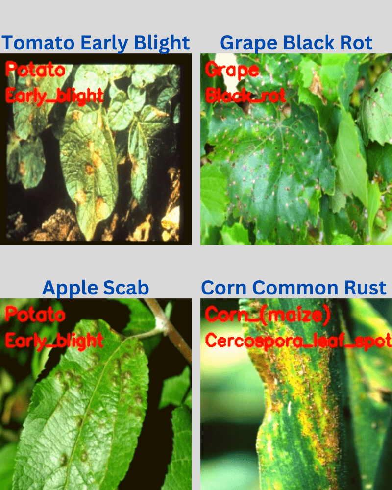
The results are very interesting. Also, they somewhat do not resonate with the test accuracy that we obtained above.

In the above results, only one prediction is entirely correct, that is the grape with black rot. The corn (maize) with Cercospora leaf spot is partially correct as only the prediction of the corn plant is correct. Finally, the other two predictions are entirely wrong. This is because the EfficientNetB0 model is predicting both, apple scab and tomato early blight as potato with early blight.

Current Issues and Further Improvements

There are a few explanations for the below-average performance of the EfficientNetB0 model even after training it on the PlantVillage disease recognition dataset. This may be because all the images in the PlantVillage dataset are captured in a controlled environment. Further, all the images have almost the same background. This means the model does not get to learn diverse surrounding contexts. Such models may perform well on the test set as it is sampled from the same dataset. But when inferencing on images with different backgrounds, it fails.

We can surely improve this. There is another dataset available for plant disease recognition. It is the PlantDoc dataset. This dataset contains images of healthy and diseased leaves in their natural surroundings. In the next post, we will carry on with our experiments of Deep Learning and AI for Plant Pathology using the PlantDoc dataset.

Summary and Conclusion

We covered a lot of ground in this post. We started with the exploration of the PlantVillage dataset for disease recognition. After training three different deep convolutional neural networks on the dataset, we tested them and also ran inference on real-life images. This gave us more insights into what issues can arise due to the dataset on which the model has been trained. We also discussed how to tackle it. I hope that this blog post was insightful for you.

If you have any doubts, thoughts, or suggestions, please leave them in the comment section. I will surely address them.

You can contact me using the Contact section. You can also find me on LinkedIn, and Twitter.

References

• PlantVillage website
• Images used for inference:
  • apple_scab.jpg
  • tomato_blight.jpg
  • corn_common_rust.jpg
  • grape_black_rot.jpg