Brain MRI Classification using PyTorch EfficientNetB0

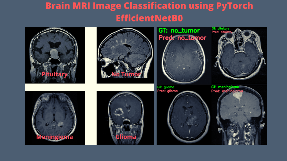
In this tutorial, we will use the PyTorch EfficientNetB0 model for brain MRI image classification.

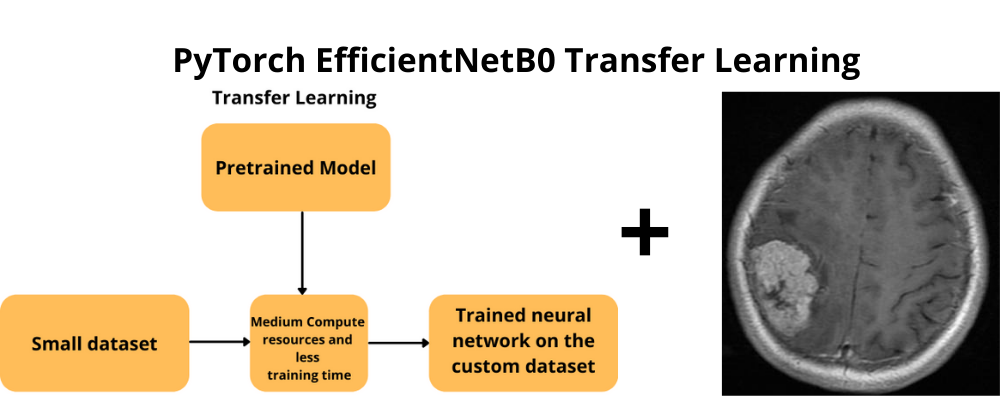
In the previous tutorial, we saw how to use the EfficientNetB0 model with the PyTorch deep learning framework for transfer learning. To show the power of transfer learning and fine-tuning, we trained the model on a very small Chess Pieces image dataset. By the end of that tutorial, we were able to conclude that even the smallest of the EfficientNet models perform really well. Even when the dataset has only a few hundred images.

To be fair, the chess pieces images dataset was not very complex. The mediocre result was mainly because of the small dataset. And the model can perform even better if we use even more augmentations. But what about more complex datasets? Like medical imaging datasets? That is what we will be testing in this tutorial. Medical image datasets always pose a greater challenge for deep learning models. The main reason is that the images are out of domain from general benchmarking datasets like ImageNet. Still, deep learning image classification models have come a long way. In fact, the EfficientNet models are some of the best out there. So, let’s see how they perform on these images.

We will cover the following topics in this tutorial.

• We will start with the exploration of the Brain Tumor MRI Dataset.
• Then we will get to know the directory structure for this project.
• After that we will move into the coding part. Here, we will write the code to train the EfficientNetB0 model on this dataset. We will use transfer learning and fine-tuning.

The Brain MRI Dataset

For the Brain MRI Classification using Pytorch EfficientNetB0, we choose this dataset from Kaggle.

The Brain Tumor MRI Dataset is a collection of brain MRI images containing four different classes.

• glioma 
• meningioma 
• no tumor
• pituitary

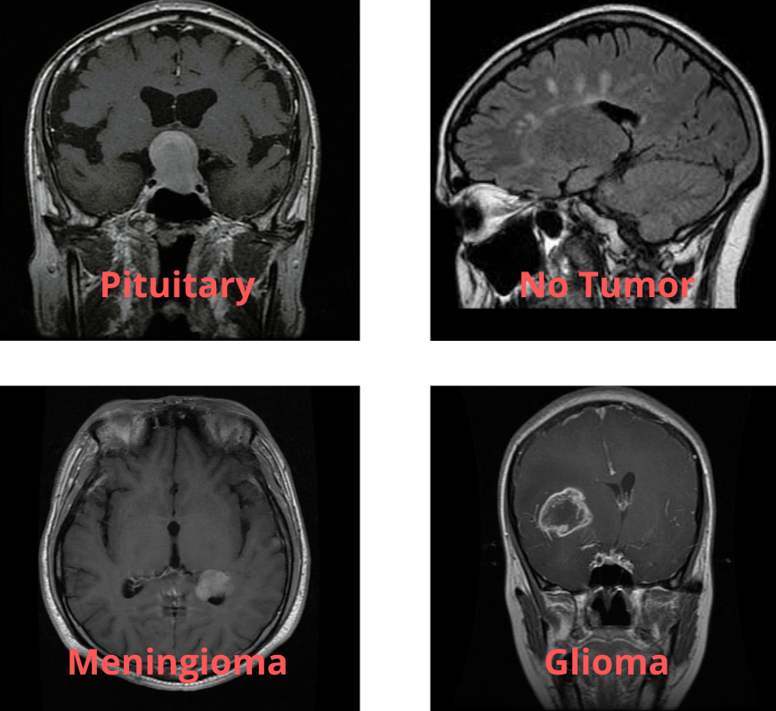
Out of the four classes, glioma, meningioma, and pituitary indicate that there is a tumor present in the MRI image. While no tumor means that there is no tumor in the brain MRI image.

The dataset from Kaggle contains 5712 training images and 1311 testing images. If you take a look at the structure, then all the images are present inside their respective class directories in the Training and Testing folders. But we will change the structure a bit.

Our final dataset structure looks something like this.

├── test_images
│   ├── glioma.jpg
│   ├── meningioma.jpg
│   ├── no_tumor.jpg
│   └── pituitary.jpg
├── training
│   ├── glioma
│   ├── meningioma
│   ├── notumor
│   └── pituitary
└── validation
    ├── glioma
    ├── meningioma
    ├── notumor
    └── pituitary

We have renamed the Training and Testing folders as training and validation. Also, we have taken four images from each class of the validation folder and put them in the test_images folder to be used for inference after training our model. The names of these images indicate the class they belong to. The inference images are not part of the training or validation set. They have been removed from those folders.

You need not worry about structuring the dataset like this. When downloading the zip file for this tutorial, you will already have the dataset in the above format.

The Directory Structure

The directory structure for the tutorial is pretty straightforward as well.

├── input
│   ├── test_images
│   │   ├── glioma.jpg
│   │   ├── meningioma.jpg
│   │   ├── no_tumor.jpg
│   │   └── pituitary.jpg
│   ├── training
│   │   ├── glioma [1321 entries exceeds filelimit, not opening dir]
│   │   ├── meningioma [1339 entries exceeds filelimit, not opening dir]
│   │   ├── notumor [1595 entries exceeds filelimit, not opening dir]
│   │   └── pituitary [1457 entries exceeds filelimit, not opening dir]
│   └── validation
│       ├── glioma [299 entries exceeds filelimit, not opening dir]
│       ├── meningioma [305 entries exceeds filelimit, not opening dir]
│       ├── notumor [404 entries exceeds filelimit, not opening dir]
│       └── pituitary [299 entries exceeds filelimit, not opening dir]
├── outputs [7 entries exceeds filelimit, not opening dir]
└── src
    ├── datasets.py
    ├── inference.py
    ├── model.py
    ├── train.py
    └── utils.py

• Inside the input directory we have the training and validation dataset along with the test images as described in the previous section.
• The outputs directory will contain the accuracy and loss graphs for training and validation, the trained model and also the inference image resutls.
• And the src directory contains all the Python files that we need for this tutorial/project.

If you download the zip file for this tutorial, then you will get all the folders and files in place along with the dataset. You will just have to follow through with this tutorial and understand the code before executing it.

The PyTorch Version

If you wish to execute all the code in this tutorial on your local system, then you need PyTorch version >= 1.10. As the EfficientNet pretrained models are only available starting from PyTorch version 1.10. You can install/upgrade from here.

PyTorch EfficientNetB0 Model for Brain MRI Image Classification

Let’s start with the coding part of the tutorial now. The code in this post will remain very similar to the previous one. There will be only minor changes in the dataset preparation code and the number of classes in the PyTorch EfficientNetB0 model. For that reason, we will only get into the details of the post where strictly necessary. Also, the code here is very similar to many other image classification projects using PyTorch. Therefore, most of the things will be pretty straightforward.

Also, note that all the Python code files are present inside the src directory.

The Helper Functions

For the helper functions, we will write the code to save the model and save the loss and accuracy graphs to disk. All these will be saved in the outputs folder.

The code for the helper functions will go into the utils.py file.

import torch
import matplotlib
import matplotlib.pyplot as plt

matplotlib.style.use('ggplot')

def save_model(epochs, model, optimizer, criterion):
    """
    Function to save the trained model to disk.
    """
    torch.save({
                'epoch': epochs,
                'model_state_dict': model.state_dict(),
                'optimizer_state_dict': optimizer.state_dict(),
                'loss': criterion,
                }, f"../outputs/model.pth")

def save_plots(train_acc, valid_acc, train_loss, valid_loss):
    """
    Function to save the loss and accuracy plots to disk.
    """
    # accuracy plots
    plt.figure(figsize=(10, 7))
    plt.plot(
        train_acc, color='green', linestyle='-', 
        label='train accuracy'
    )
    plt.plot(
        valid_acc, color='blue', linestyle='-', 
        label='validataion accuracy'
    )
    plt.xlabel('Epochs')
    plt.ylabel('Accuracy')
    plt.legend()
    plt.savefig(f"../outputs/accuracy.png")
    
    # loss plots
    plt.figure(figsize=(10, 7))
    plt.plot(
        train_loss, color='orange', linestyle='-', 
        label='train loss'
    )
    plt.plot(
        valid_loss, color='red', linestyle='-', 
        label='validataion loss'
    )
    plt.xlabel('Epochs')
    plt.ylabel('Loss')
    plt.legend()
    plt.savefig(f"../outputs/loss.png")

• The save_model() function saves the trained model to disk. We save the information about the number of epochs trained for, the optimizer state, and also the loss function information. This will be helpful if we will want to resume training anytime in the future.
• The save_plots() is a simple function which plots the accuracy and loss graphs for training and validation, then saves them to disk.

Preparing the Dataset

As we already have the training and validation images inside the respective directories, so the dataset preparation will become simpler.

The code here will go into the datasets.py file.

Starting with the imports and defining the necessary constants.

from torchvision import datasets, transforms
from torch.utils.data import DataLoader

# Required constants.
TRAIN_DIR = '../input/training'
VALID_DIR = '../input/validation'
IMAGE_SIZE = 224 # Image size of resize when applying transforms.
BATCH_SIZE = 32 
NUM_WORKERS = 4 # Number of parallel processes for data preparation.

We have the path to the training and validation images, the image size to resize to when applying the transforms, batch size, and the number of workers for data preprocessing.

Next, we define the functions for the training and the validation transforms.

# Training transforms
def get_train_transform(IMAGE_SIZE):
    train_transform = transforms.Compose([
        transforms.Resize((IMAGE_SIZE, IMAGE_SIZE)),
        transforms.RandomHorizontalFlip(p=0.5),
        transforms.RandomVerticalFlip(p=0.5),
        transforms.GaussianBlur(kernel_size=(5, 9), sigma=(0.1, 5)),
        transforms.RandomAdjustSharpness(sharpness_factor=2, p=0.5),
        transforms.ToTensor(),
        transforms.Normalize(
            mean=[0.485, 0.456, 0.406],
            std=[0.229, 0.224, 0.225]
            )
    ])
    return train_transform

# Validation transforms
def get_valid_transform(IMAGE_SIZE):
    valid_transform = transforms.Compose([
        transforms.Resize((IMAGE_SIZE, IMAGE_SIZE)),
        transforms.ToTensor(),
        transforms.Normalize(
            mean=[0.485, 0.456, 0.406],
            std=[0.229, 0.224, 0.225]
            )
    ])
    return valid_transform

For the training transforms we apply the following augmentations:

• RandomHorizontalFlip: Flipping the image horizontally randomly.
• RandomVerticalFlip: Randomly flipping the image vertically.
• GaussianBlur: Applying Gaussian blurring to the image.
• RandomAdjustSharpness: Changing the sharpness of the image randomly.

Note that we do not apply color or contrast augmentation here. The reason is that it may affect how the MRI images should appear in a negative way and the model might miss out on the original color information that it needs for proper learning. Although, it can be taken up as a future task to experiment with.

We are applying the ImageNet normalization values for both, training and validation transform. This is because we will use a pretrained EfficientNetB0 model here.

Finally, we write the code to prepare the datasets and the data loaders.

def get_datasets():
    """
    Function to prepare the Datasets.

    Returns the training and validation datasets along 
    with the class names.
    """
    dataset_train = datasets.ImageFolder(
        TRAIN_DIR, 
        transform=(get_train_transform(IMAGE_SIZE))
    )
    dataset_valid = datasets.ImageFolder(
        VALID_DIR, 
        transform=(get_valid_transform(IMAGE_SIZE))
    )
    return dataset_train, dataset_valid, dataset_train.classes

def get_data_loaders(dataset_train, dataset_valid):
    """
    Prepares the training and validation data loaders.

    :param dataset_train: The training dataset.
    :param dataset_valid: The validation dataset.

    Returns the training and validation data loaders.
    """
    train_loader = DataLoader(
        dataset_train, batch_size=BATCH_SIZE, 
        shuffle=True, num_workers=NUM_WORKERS
    )
    valid_loader = DataLoader(
        dataset_valid, batch_size=BATCH_SIZE, 
        shuffle=False, num_workers=NUM_WORKERS
    )
    return train_loader, valid_loader 

The get_datasets() function prepares the training and validation datasets and returns them along with the class names.

The get_data_loaders() function takes in the datasets as parameters and prepares the training and validation data loaders.

The EfficientNetB0 Model

We can easily load the pretrained EfficientNetB0 model from torchvision.models. And that is what we will do here as well.

The code to prepare the model will go into the model.py file.

import torchvision.models as models
import torch.nn as nn

def build_model(pretrained=True, fine_tune=True, num_classes=10):
    if pretrained:
        print('[INFO]: Loading pre-trained weights')
    else:
        print('[INFO]: Not loading pre-trained weights')
    model = models.efficientnet_b0(pretrained=pretrained)

    if fine_tune:
        print('[INFO]: Fine-tuning all layers...')
        for params in model.parameters():
            params.requires_grad = True
    elif not fine_tune:
        print('[INFO]: Freezing hidden layers...')
        for params in model.parameters():
            params.requires_grad = False

    # Change the final classification head.
    model.classifier[1] = nn.Linear(in_features=1280, out_features=num_classes)
    return model

On line 21, we are just changing the number of classes as per our dataset here. That’s it. Our PyTorch EfficientNet model for brain MRI image classification is ready. Although it is worth noting that we will be loading the pretrained weights and fine-tuning all the layers as well. When the model was trained on the ImageNet dataset, it is very unlikely that it has seen any brain MRI images. So, by loading pretrained ImageNet weights, we already start at a good place. Then we slowly update the weights according to our dataset.

The Training Script

This is the final script that we need to write the code before we start the training.

The code for the training script will go into the train.py file.

Starting with the imports and constructing the argument parser.

import torch
import argparse
import torch.nn as nn
import torch.optim as optim
import time

from tqdm.auto import tqdm

from model import build_model
from datasets import get_datasets, get_data_loaders
from utils import save_model, save_plots

# Construct the argument parser.
parser = argparse.ArgumentParser()
parser.add_argument(
    '-e', '--epochs', type=int, default=20,
    help='Number of epochs to train our network for'
)
parser.add_argument(
    '-lr', '--learning-rate', type=float,
    dest='learning_rate', default=0.0001,
    help='Learning rate for training the model'
)
args = vars(parser.parse_args())

We have two flags for the argument parser:

• --epochs: The number of epochs to train for.
• --learning-rate: The learning rate for the optimizer.

The Training and Validation Functions

First, the training function.

# Training function.
def train(model, trainloader, optimizer, criterion):
    model.train()
    print('Training')
    train_running_loss = 0.0
    train_running_correct = 0
    counter = 0
    for i, data in tqdm(enumerate(trainloader), total=len(trainloader)):
        counter += 1
        image, labels = data
        image = image.to(device)
        labels = labels.to(device)
        optimizer.zero_grad()
        # Forward pass.
        outputs = model(image)
        # Calculate the loss.
        loss = criterion(outputs, labels)
        train_running_loss += loss.item()
        # Calculate the accuracy.
        _, preds = torch.max(outputs.data, 1)
        train_running_correct += (preds == labels).sum().item()
        # Backpropagation
        loss.backward()
        # Update the weights.
        optimizer.step()
    
    # Loss and accuracy for the complete epoch.
    epoch_loss = train_running_loss / counter
    epoch_acc = 100. * (train_running_correct / len(trainloader.dataset))
    return epoch_loss, epoch_acc

It returns the loss and accuracy for each epoch.

Now, the validation function, which returns the accuracy and loss values as well.

# Validation function.
def validate(model, testloader, criterion):
    model.eval()
    print('Validation')
    valid_running_loss = 0.0
    valid_running_correct = 0
    counter = 0
    with torch.no_grad():
        for i, data in tqdm(enumerate(testloader), total=len(testloader)):
            counter += 1
            
            image, labels = data
            image = image.to(device)
            labels = labels.to(device)
            # Forward pass.
            outputs = model(image)
            # Calculate the loss.
            loss = criterion(outputs, labels)
            valid_running_loss += loss.item()
            # Calculate the accuracy.
            _, preds = torch.max(outputs.data, 1)
            valid_running_correct += (preds == labels).sum().item()
        
    # Loss and accuracy for the complete epoch.
    epoch_loss = valid_running_loss / counter
    epoch_acc = 100. * (valid_running_correct / len(testloader.dataset))
    return epoch_loss, epoch_acc

The Main Code Block

The final part of the training script is writing the main code block.

if __name__ == '__main__':
    # Load the training and validation datasets.
    dataset_train, dataset_valid, dataset_classes = get_datasets()
    print(f"[INFO]: Number of training images: {len(dataset_train)}")
    print(f"[INFO]: Number of validation images: {len(dataset_valid)}")
    print(f"[INFO]: Class names: {dataset_classes}\n")
    # Load the training and validation data loaders.
    train_loader, valid_loader = get_data_loaders(dataset_train, dataset_valid)

    # Learning_parameters. 
    lr = args['learning_rate']
    epochs = args['epochs']
    device = ('cuda' if torch.cuda.is_available() else 'cpu')
    print(f"Computation device: {device}")
    print(f"Learning rate: {lr}")
    print(f"Epochs to train for: {epochs}\n")

    model = build_model(
        pretrained=True,
        fine_tune=True, 
        num_classes=len(dataset_classes)
    ).to(device)
    
    # Total parameters and trainable parameters.
    total_params = sum(p.numel() for p in model.parameters())
    print(f"{total_params:,} total parameters.")
    total_trainable_params = sum(
        p.numel() for p in model.parameters() if p.requires_grad)
    print(f"{total_trainable_params:,} training parameters.")

    # Optimizer.
    optimizer = optim.Adam(model.parameters(), lr=lr)
    # Loss function.
    criterion = nn.CrossEntropyLoss()

    # Lists to keep track of losses and accuracies.
    train_loss, valid_loss = [], []
    train_acc, valid_acc = [], []
    # Start the training.
    for epoch in range(epochs):
        print(f"[INFO]: Epoch {epoch+1} of {epochs}")
        train_epoch_loss, train_epoch_acc = train(model, train_loader, 
                                                optimizer, criterion)
        valid_epoch_loss, valid_epoch_acc = validate(model, valid_loader,  
                                                    criterion)
        train_loss.append(train_epoch_loss)
        valid_loss.append(valid_epoch_loss)
        train_acc.append(train_epoch_acc)
        valid_acc.append(valid_epoch_acc)
        print(f"Training loss: {train_epoch_loss:.3f}, training acc: {train_epoch_acc:.3f}")
        print(f"Validation loss: {valid_epoch_loss:.3f}, validation acc: {valid_epoch_acc:.3f}")
        print('-'*50)
        time.sleep(5)
        
    # Save the trained model weights.
    save_model(epochs, model, optimizer, criterion)
    # Save the loss and accuracy plots.
    save_plots(train_acc, valid_acc, train_loss, valid_loss)
    print('TRAINING COMPLETE')

The above main code block includes the following things:

• We start with preparing the datasets and data loaders (lines 84 to 89).
• After the learning parameters, we initialize the model on line 99.
• We start the training loop from line 121. After each epoch, we are printing the loss and accuracy values for both training and validation.
• After the training completes, we save the model and the graphs to disk.

This completes all the code we need for training the PyTorch EfficientNetB0 model on the brain MRI classification dataset.

Execute train.py to Start Training

Finally, we have reached the training phase in the tutorial.

You may open your terminal/command line from the src directory and execute the following command to start the training.

python train.py --epochs 35

We are training the model for 35 epochs with the default learning rate of 0.0001.

The following block shows the truncated output.

[INFO]: Number of training images: 5712
[INFO]: Number of validation images: 1307
[INFO]: Class names: ['glioma', 'meningioma', 'notumor', 'pituitary']

Computation device: cuda
Learning rate: 0.0001
Epochs to train for: 35

[INFO]: Loading pre-trained weights
[INFO]: Fine-tuning all layers...
4,012,672 total parameters.
4,012,672 training parameters.
[INFO]: Epoch 1 of 35
Training
100%|██████████████████████████████████████████████████████████████████| 179/179 [00:12<00:00, 14.79it/s]
Validation
100%|████████████████████████████████████████████████████████████████████| 41/41 [00:00<00:00, 42.34it/s]
Training loss: 0.498, training acc: 83.718
Validation loss: 0.222, validation acc: 91.890
--------------------------------------------------
...
[INFO]: Epoch 35 of 35
Training
100%|██████████████████████████████████████████████████████████████████| 179/179 [00:11<00:00, 15.39it/s]
Validation
100%|████████████████████████████████████████████████████████████████████| 41/41 [00:00<00:00, 42.93it/s]
Training loss: 0.011, training acc: 99.667
Validation loss: 0.009, validation acc: 99.694
--------------------------------------------------
TRAINING COMPLETE

After the last epoch, we have a validation accuracy of more than 99% and a validation loss of 0.009. This looks good.

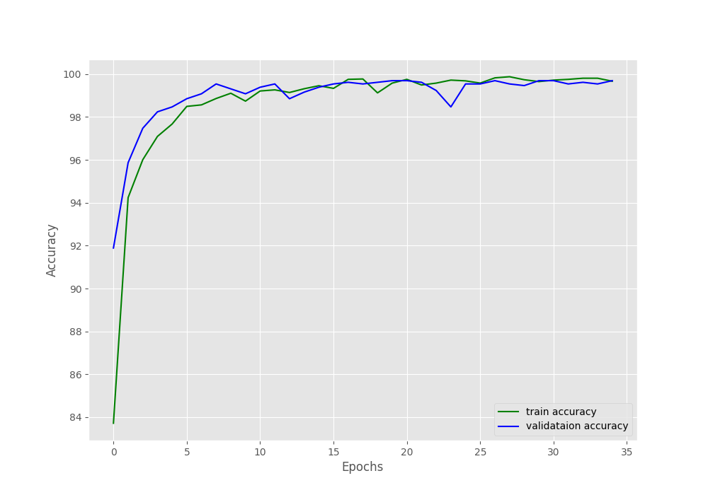
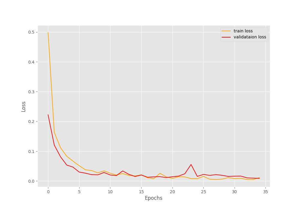
The accuracy and loss graphs also look pretty good. For both, training and validation, there is not much fluctuation in the plots.

We will get to know how well the model has learned once we run the inference on the test images.

The Inference Script

In this section, we will write the inference code which we will use to predict the classes on unseen Brain MRI images using the trained model.

The code in this section will go into the inference.py script.

import torch
import cv2
import numpy as np
import glob as glob
import os

from model import build_model
from torchvision import transforms

# Constants.
DATA_PATH = '../input/test_images'
IMAGE_SIZE = 224
DEVICE = 'cpu'

# Class names.
class_names = ['glioma', 'meningioma', 'no_tumor', 'pituitary']

Above, we first import all the required modules. Then we define a few constants from line 11 and a list containing the class names on line 16.

Next, we initialize the model and load the trained weights.

# Load the trained model.
model = build_model(pretrained=False, fine_tune=False, num_classes=4)
checkpoint = torch.load('../outputs/model.pth', map_location=DEVICE)
print('Loading trained model weights...')
model.load_state_dict(checkpoint['model_state_dict'])

The final part is iterating over all the test images and running the inference on each of them.

# Get all the test image paths.
all_image_paths = glob.glob(f"{DATA_PATH}/*")
# Iterate over all the images and do forward pass.
for image_path in all_image_paths:
    # Get the ground truth class name from the image path.
    gt_class_name = image_path.split(os.path.sep)[-1].split('.')[0]
    # Read the image and create a copy.
    image = cv2.imread(image_path)
    orig_image = image.copy()
    
    # Preprocess the image
    image = cv2.cvtColor(image, cv2.COLOR_BGR2RGB)
    transform = transforms.Compose([
        transforms.ToPILImage(),
        transforms.Resize((IMAGE_SIZE, IMAGE_SIZE)),
        transforms.ToTensor(),
        transforms.Normalize(
            mean=[0.485, 0.456, 0.406],
            std=[0.229, 0.224, 0.225]
        )
    ])
    image = transform(image)
    image = torch.unsqueeze(image, 0)
    image = image.to(DEVICE)
    
    # Forward pass throught the image.
    outputs = model(image)
    outputs = outputs.detach().numpy()
    pred_class_name = class_names[np.argmax(outputs[0])]
    print(f"GT: {gt_class_name}, Pred: {pred_class_name.lower()}")
    # Annotate the image with ground truth.
    cv2.putText(
        orig_image, f"GT: {gt_class_name}",
        (10, 25), cv2.FONT_HERSHEY_SIMPLEX,
        0.8, (0, 255, 0), 2, lineType=cv2.LINE_AA
    )
    # Annotate the image with prediction.
    cv2.putText(
        orig_image, f"Pred: {pred_class_name.lower()}",
        (10, 55), cv2.FONT_HERSHEY_SIMPLEX,
        0.8, (100, 100, 225), 2, lineType=cv2.LINE_AA
    ) 
    cv2.imshow('Result', orig_image)
    cv2.waitKey(0)
    cv2.imwrite(f"../outputs/{gt_class_name}.png", orig_image)

We store all the test image paths in the all_image_paths list. Then we start to iterate over these paths from line 25.

The gt_class_name on line 27 stores the ground truth class of the current image. Starting from line 29, we read the image, create a copy of it, change the color to RGB format, and apply the preprocessing transforms. The forward pass happens on line 48. On line 50, pred_class_name stores the predicted class of the image. Then we print the ground truth and predicted class name and annotate the original image with the same. Finally, we show the result and save it to disk.

Execute inference.py

Let’s check how our model performs in the test images.

python inference.py 

The following output is from the terminal.

[INFO]: Not loading pre-trained weights
[INFO]: Freezing hidden layers...
Loading trained model weights...
GT: glioma, Pred: glioma
GT: pituitary, Pred: pituitary
GT: no_tumor, Pred: no_tumor
GT: meningioma, Pred: meningioma

And the output image results.

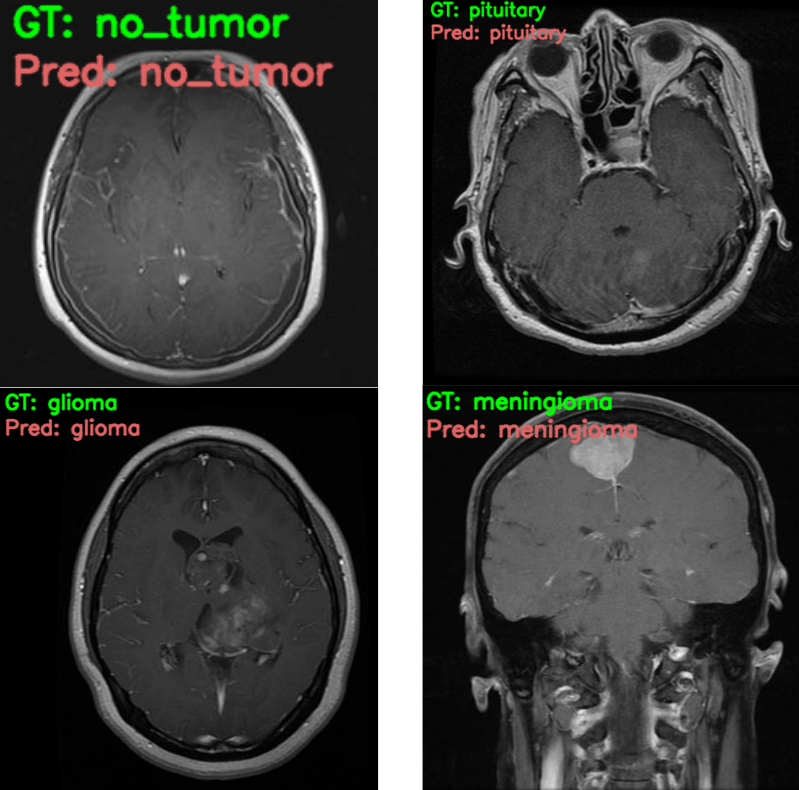
The model is able to predict all the image classes correctly. That’s great. It has learned the features of the images from the dataset really well. Most probably, any other model from scratch with around 4 million parameters would have never been able to achieve such results. This really shows the power of both, transfer learning and the EfficientNetB0 model.

Further Experiments

There are a few things that we may do to improve the overall project and performance of the model.

You may have observed that all the MRI images have black pixels around them and the brain MRI is mostly at the center.

This means that the model needs to focus on that MRI part only and we do not need the black borders/pixels. Most probably, we can devise a way to safely crop out the black pixels and train the model again. This is very likely to improve performance. Do let us know in the comment section if you try this experiment.

Summary and Conclusion

In this tutorial, we carried out Brain MRI Classification using PyTorch EfficientNetB0. We started with exploring the dataset, then trained the EfficientNetB0 model, and finally, ran the inference. In the end, we also discussed some possible ways to improve the model’s performance further. I hope that this tutorial was helpful to you.

If you have any doubts, thoughts, or suggestions, please leave them in the comment section. I will surely address them.

You can contact me using the Contact section. You can also find me on LinkedIn, and Twitter.