Faster Image Augmentation in TensorFlow using Keras Layers

In this tutorial, we will learn how to do faster image augmentation in TensorFlow, ON GPU!

Data augmentation has been an integral part of training deep learning models, especially in computer vision tasks. In TensorFlow, the ImageDataGenerator class provides a host of augmentation techniques that we can use. This comes as a savior to train models for achieving higher accuracy when dealing with small datasets. Still, we can use data augmentation techniques with larger datasets to train even better models. But there is one big drawback to using the augmentations from ImageDataGenerator class. All the augmentation happens on the CPU while mostly, the training happens on the CPU. This can be a big bottleneck at times when the model has to wait for the data to be preprocessed before it can be fed into the layers. In this post, we will see how to overcome that using TensorFlow and Keras.

We will cover the following topics in this tutorial.

• We will start with a short discussion on image data augmentation.
  • How is it generally done using TensorFlow and Keras?
  • What new thing can we do to improve performance?
• Then we will get to know the dataset and directory structure for this tutorial.
• Next, we will jump into the coding part of the tutorial.

Image Data Augmentation using TensorFlow and Keras

As we know, image augmentation with the TensorFlow ImageDataGenerator can be very slow. It can even increase the per epoch training time by two-fold at times. This is not desirable when dealing with huge datasets. When we have the right GPU and a good model in place, we do not want that the preprocessing should slow down the training. This mainly happens because the augmentations take place on the CPU.

Image Augmentation using tf.keras.layers

With the recent versions of TensorFlow, we are able to offload much of this CPU processing part onto the GPU. Now, with tf.keras.layers some of the image augmentation techniques can be applied on the fly just before being fed into the neural network. As this happens within the tf.keras.layers module, if we train our model on the GPU, then the augmentation will also happen on the GPU.

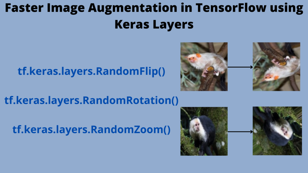
As of now, we have a pretty decent collection of image augmentation that we can carry out using tf.keras.layers. These include (without getting into the technical details):

• tf.keras.layers.RandomFlip: For randomly flipping the image horizontally and vertically during training.
• tf.keras.layers.RandomRotation: Randomly rotates the image during training.
• tf.keras.layers.RandomZoom: Randomly zooms the image during training.
• tf.keras.layers.RandomContrast: For adjusting the contrast of the image during training.
• tf.keras.layers.RandomCrop: For random cropping of the image.
• tf.keras.layers.RandomHeight: Randomly varies image height during training.
• tf.keras.layers.RandomWidth: Randomly varies image width during training.

All of the above layers can act as both preprocessing and augmentation layers during training. There are a few which can only act as image preprocessing layers.

• tf.keras.layers.Rescaling: A preprocessing layer which rescales input values to a new range.
• tf.keras.layers.Reshape: Let’s us reshape the input into another shape.
• tf.keras.layers.Resizing: For resizing images.

You can find all the preprocessing and augmentation layers here.

The Dataset

In this tutorial, we will be using the 10 Monkey Species dataset from Kaggle.

The dataset contains images of 10 different monkey species.

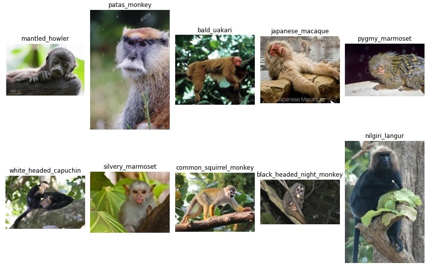
The following image shows a few more details about the dataset.

As you can see we have the Label column from n0 to n9. The other columns show the common name, the Latin name, number of training, and validation images. The training and validation images are inside the respective class folders which are named from n0 to n9.

There are about 1400 images in total in the dataset.

Before moving ahead in the tutorial, I recommend that you download the dataset if you intend to execute the code locally in your system.

The Directory Structure

Let’s check out the directory structure for the tutorial now.

.
├── input
│   ├── training
│   │   └── training
│   │       ├── n0 [105 entries exceeds filelimit, not opening dir]
│   │       ├── n1 [111 entries exceeds filelimit, not opening dir]
│   │       ├── n2 [110 entries exceeds filelimit, not opening dir]
│   │       ├── n3 [122 entries exceeds filelimit, not opening dir]
│   │       ├── n4 [105 entries exceeds filelimit, not opening dir]
│   │       ├── n5 [113 entries exceeds filelimit, not opening dir]
│   │       ├── n6 [106 entries exceeds filelimit, not opening dir]
│   │       ├── n7 [114 entries exceeds filelimit, not opening dir]
│   │       ├── n8 [106 entries exceeds filelimit, not opening dir]
│   │       └── n9 [106 entries exceeds filelimit, not opening dir]
│   ├── validation
│   │   └── validation
│   │       ├── n0 [26 entries exceeds filelimit, not opening dir]
│   │       ├── n1 [28 entries exceeds filelimit, not opening dir]
│   │       ├── n2 [27 entries exceeds filelimit, not opening dir]
│   │       ├── n3 [30 entries exceeds filelimit, not opening dir]
│   │       ├── n4 [26 entries exceeds filelimit, not opening dir]
│   │       ├── n5 [28 entries exceeds filelimit, not opening dir]
│   │       ├── n6 [26 entries exceeds filelimit, not opening dir]
│   │       ├── n7 [28 entries exceeds filelimit, not opening dir]
│   │       ├── n8 [27 entries exceeds filelimit, not opening dir]
│   │       └── n9 [26 entries exceeds filelimit, not opening dir]
│   └── monkey_labels.txt
├── outputs
│   ├── accuracy.png
│   └── loss.png
├── src
│   ├── model.py
│   ├── train.py
│   └── utils.py

• The input directory contains the training and validation data inside the respective class directories.
• The outputs directory will contain the accuracy and loss graphs.
• And the src directory holds the three Python files that we need for the tutorial.

For now, you can ignore the monkey_labels.txt file as we do not need that in this tutorial.

The TensorFlow Version

This tutorial is based on TensorFlow version 2.6.2. You can install/upgrade your TensorFlow version here.

Faster Image Augmentation in TensorFlow

Now we will start with the coding part. We have three Python files and will write the code for each in their respective sections.

Let’s write the code in each file in the following order:

• utils.py
• model.py
• train.py

The Python files will stay inside the src directory.

The Helper Functions

We will start with writing a few helper functions. These will go into the utils.py file.

Let’s start with the import statements and the first function.

import matplotlib.pyplot as plt
import tensorflow as tf

plt.style.use('ggplot')

def prepare_batches(
    TRAINING_DATA_DIR, VALID_DATA_DIR, 
    IMAGE_SHAPE, BATCH_SIZE
):
    train_datagen = tf.keras.preprocessing.image.ImageDataGenerator()
    valid_datagen = tf.keras.preprocessing.image.ImageDataGenerator()

    train_batches = train_datagen.flow_from_directory(
    TRAINING_DATA_DIR,
    shuffle=True,
    target_size=IMAGE_SHAPE,
    batch_size=BATCH_SIZE
    )
    valid_batches = valid_datagen.flow_from_directory(
        VALID_DATA_DIR,
        shuffle=False,
        target_size=IMAGE_SHAPE,
        batch_size=BATCH_SIZE
    )
    return train_batches, valid_batches

We need matplotlib for plotting of accuracy and loss graphs and tensorflow for preparing the dataset.

The prepare_batches function starting from line 6 prepares the training and validation data batches. It accepts the paths to the training and validation data, image size to resize to, and batch size as parameters. You may notice that the train_datagen and valid_datagen are the same. This is because we are not doing any preprocessing or augmentation here, not even the rescaling of images. We will do everything in the model layers. We prepare the training and validation batches on lines 13 and 19 respectively.

The next function is for saving the plots for loss and accuracy graphs.

def save_plots(train_acc, valid_acc, train_loss, valid_loss):
    """
    Function to save the loss and accuracy plots to disk.
    """
    # Accuracy plots.
    plt.figure(figsize=(12, 9))
    plt.plot(
        train_acc, color='green', linestyle='-', 
        label='train accuracy'
    )
    plt.plot(
        valid_acc, color='blue', linestyle='-', 
        label='validataion accuracy'
    )
    plt.xlabel('Epochs')
    plt.ylabel('Accuracy')
    plt.legend()
    plt.savefig(f"../outputs/accuracy.png")
    plt.show()
    # Loss plots.
    plt.figure(figsize=(12, 9))
    plt.plot(
        train_loss, color='orange', linestyle='-', 
        label='train loss'
    )
    plt.plot(
        valid_loss, color='red', linestyle='-', 
        label='validataion loss'
    )
    plt.xlabel('Epochs')
    plt.ylabel('Loss')
    plt.legend()
    plt.savefig(f"../outputs/loss.png")
    plt.show()

The save_plots() function accepts the training accuracy, validation accuracy, training loss, and validation loss from the history object after training. It then saves the accuracy and loss graphs inside the outputs directory.

The Neural Network Model

The neural network model that we will use is quite simple actually. But here, instead of using the Sequential model, we will create it with the functional API. Integrating the keras preprocessing/augmentation layers within a function API model is pretty straightforward and feels intuitive as well.

The model preparation code will go into the model.py file.

The following code block contains the entire model preparation function.

import tensorflow as tf

def build_model(num_classes):
    inputs = tf.keras.layers.Input(shape=(224, 224, 3))
    
    # Add the preprocessing/augmentation layers.
    x = tf.keras.layers.RandomFlip(mode='horizontal_and_vertical')(inputs)
    x = tf.keras.layers.RandomRotation(0.1)(x)
    x = tf.keras.layers.RandomZoom(0.2)(x)
    x = tf.keras.layers.Rescaling(1./255)(x)
    
    # Add the model layers.
    x = tf.keras.layers.Conv2D(
        filters=16, kernel_size=(3, 3), activation='relu'
    )(x)
    x = tf.keras.layers.MaxPooling2D(pool_size=(2, 2), strides=2)(x)
    x = tf.keras.layers.Conv2D(
        filters=32, kernel_size=(3, 3), activation='relu'
    )(x)
    x = tf.keras.layers.MaxPooling2D(pool_size=(2, 2), strides=2)(x)
    x = tf.keras.layers.Conv2D(
        filters=64, kernel_size=(3, 3), activation='relu'
    )(x)
    x = tf.keras.layers.MaxPooling2D(pool_size=(2, 2), strides=2)(x)
    x = tf.keras.layers.Flatten()(x)
    x = tf.keras.layers.Dense(128, activation='relu')(x)
    output = tf.keras.layers.Dense(num_classes, activation='softmax')(x)
    model = tf.keras.Model(inputs, output)
    return model

Let’s check out what is happening here:

• As usual, we start with the input layer on line 4.
• From line 7 to 10, we have the augmentation and preprocessing layers using tf.keras.layers.
  • We use RandomFlip where the mode is horizontal_and_vertical indicating that both horizontal and vertical flipping will be applied.
  • The RandomRotation has a factor of 0.1 indicating the image will be rotated by 10%, around 36 degrees.
  • And then we have the RandomZoom with a factor of 0.2.
• We have the neural network model layers from line 13. There are 2D convolutional layers with 16, 32, and 64 output channels respectively. 2D max-pooling layers follow each of the convolutional layers. After flattening the convolutional features, we apply the Dense layer with 128 units.
• The final Dense layer on line 27 has num_classes number of units with softmax activation.

The above model has around 5.5 million trainable parameters. It may not be the best model but it is good enough to try out the tf.keras.layers for the first time.

The Training Script

The training script is going to be the easiest to write perhaps. It is the final executable Python file and will contain:

• Preparation of the data batches.
• Preparation of the model.
• And the fit() method for training.

All this code will go into the train.py file.

Let’s start with the import statements and a few necessary constants.

import tensorflow as tf

from utils import prepare_batches, save_plots
from model import build_model

# Constants and paths
IMAGE_SHAPE = (224, 224) # For resizing
TRAINING_DATA_DIR = '../input/training/training/'
VALID_DATA_DIR = '../input/validation/validation/'
BATCH_SIZE = 32
EPOCHS = 80

We import the required functions from utils and model modules. Then we initialize a few constants defining the image size, the training and validation data paths, the batch size, and the number of epochs to train for.

Next, we prepare the training & validation data batches, and the model as well.

# Prepare the data batches.
train_batches, valid_batches = prepare_batches(
    TRAINING_DATA_DIR, VALID_DATA_DIR, IMAGE_SHAPE, BATCH_SIZE
)

# Prepare and compile the model.
model = build_model(num_classes=10)
model.compile(
    optimizer=tf.keras.optimizers.Adam(lr=0.0001),
    loss=tf.keras.losses.CategoricalCrossentropy(from_logits=False),
    metrics=['accuracy']
)
print(model.summary())

While compiling the model, we use the CategoricalCrossentropy loss function and the accuracy metrics. Note that we are using the learning rate of 0.0001 here. Using a higher learning rate was causing the model to overfit very soon.

The final step is training the model using the fit() method and saving the accuracy and loss graphs at the end.

# Train the model.
history = model.fit(
    train_batches,
    steps_per_epoch=train_batches.samples // BATCH_SIZE,
    epochs=EPOCHS,
    validation_data=valid_batches,
    validation_steps= valid_batches.samples // BATCH_SIZE,
    verbose=1,
    workers=4,
    use_multiprocessing=True
)

# Save the plots to disk.
train_loss = history.history['loss']
train_acc = history.history['accuracy']
valid_loss = history.history['val_loss']
valid_acc = history.history['val_accuracy']
save_plots(train_acc, valid_acc, train_loss, valid_loss)

In the fit() method, we are using workers=4, and use_multiprocessing=True to speed up the training even further in terms of time. This allows TensorFlow to use different CPU processes to prepare the data beforehand while the model is iterating through the current data batches. Typically, this should help to achieve 2x more training speed per epoch at times. The steps_per_epoch and validation_steps are optional arguments. If not provided, the fit() method will be able to infer it automatically from the batch size and the total number of training and validation samples.

Finally, we extract the loss and accuracy values from the history object and pass it to the save_plots() function for the plotting to happen.

This is all the code we need to carry out Faster Image Augmentation in TensorFlow using tf.keras.layers.

Execute train.py

Now, we are all set to execute train.py and carry out the training. Open your terminal/command line in the src directory and execute the following command.

python train.py 

The following block shows the truncated output. You should see something similar to this.

Found 1098 images belonging to 10 classes.
Found 272 images belonging to 10 classes.

Model: "model"
_________________________________________________________________
Layer (type)                 Output Shape              Param #   
=================================================================
input_1 (InputLayer)         [(None, 224, 224, 3)]     0         
_________________________________________________________________
random_flip (RandomFlip)     (None, 224, 224, 3)       0         
_________________________________________________________________
random_rotation (RandomRotat (None, 224, 224, 3)       0         
_________________________________________________________________
random_zoom (RandomZoom)     (None, 224, 224, 3)       0         
_________________________________________________________________
rescaling (Rescaling)        (None, 224, 224, 3)       0         
_________________________________________________________________
conv2d (Conv2D)              (None, 222, 222, 16)      448       
_________________________________________________________________
max_pooling2d (MaxPooling2D) (None, 111, 111, 16)      0         
_________________________________________________________________
conv2d_1 (Conv2D)            (None, 109, 109, 32)      4640      
_________________________________________________________________
max_pooling2d_1 (MaxPooling2 (None, 54, 54, 32)        0         
_________________________________________________________________
conv2d_2 (Conv2D)            (None, 52, 52, 64)        18496     
_________________________________________________________________
max_pooling2d_2 (MaxPooling2 (None, 26, 26, 64)        0         
_________________________________________________________________
flatten (Flatten)            (None, 43264)             0         
_________________________________________________________________
dense (Dense)                (None, 128)               5537920   
_________________________________________________________________
dense_1 (Dense)              (None, 10)                1290      
=================================================================
Total params: 5,562,794
Trainable params: 5,562,794
Non-trainable params: 0
_________________________________________________________________
None

Epoch 1/80
34/34 [==============================] - 11s 165ms/step - loss: 2.2626 - accuracy: 0.1567 - val_loss: 2.1845 - val_accuracy: 0.2227
Epoch 2/80
34/34 [==============================] - 6s 143ms/step - loss: 2.0943 - accuracy: 0.2392 - val_loss: 2.0374 - val_accuracy: 0.2617
Epoch 3/80
34/34 [==============================] - 6s 162ms/step - loss: 1.9300 - accuracy: 0.2861 - val_loss: 1.9076 - val_accuracy: 0.3359
Epoch 4/80
34/34 [==============================] - 6s 146ms/step - loss: 1.8237 - accuracy: 0.3396 - val_loss: 1.8763 - val_accuracy: 0.3281
Epoch 5/80
34/34 [==============================] - 6s 147ms/step - loss: 1.7727 - accuracy: 0.3583 - val_loss: 1.8401 - val_accuracy: 0.3320
...
Epoch 76/80
34/34 [==============================] - 6s 152ms/step - loss: 0.8216 - accuracy: 0.7280 - val_loss: 1.2346 - val_accuracy: 0.6172
Epoch 77/80
34/34 [==============================] - 6s 159ms/step - loss: 0.7764 - accuracy: 0.7411 - val_loss: 1.2259 - val_accuracy: 0.6328
Epoch 78/80
34/34 [==============================] - 6s 149ms/step - loss: 0.8113 - accuracy: 0.7195 - val_loss: 1.2302 - val_accuracy: 0.6016
Epoch 79/80
34/34 [==============================] - 6s 146ms/step - loss: 0.7620 - accuracy: 0.7364 - val_loss: 1.3293 - val_accuracy: 0.5898
Epoch 80/80
34/34 [==============================] - 6s 145ms/step - loss: 0.7634 - accuracy: 0.7411 - val_loss: 1.1798 - val_accuracy: 0.6133

As you can see, the training for one epoch took somewhere around 6 seconds. This experiment was carried out on a machine with RTX 3080 GPU and i7 10th Gen CPU. Your results will vary depending on the hardware that you are using.

Although we did not carry out image augmentation using ImageDataGenerator, still with the same set of augmentations took somewhere around 3 seconds more on the same hardware. This may not seem like a big increase, but it will increase substantially when adding more augmentations. But most probably, the tf.keras.layers augmentation will still result somewhere around 6-7 seconds per epoch.

The following are the accuracy and loss graphs.

Looks like we were only able to achieve 61% validation accuracy by the end. This is because we were using augmentation with a very simple model. A better model will surely give higher accuracy.

To experiment further:

• You may add more augmentations with a bigger model and check out the training.
• You can compare the training time with ImageDataGenerator augmentation’s training time.
• Although you may not find the exact augmentations in both tf.keras.layers and ImageDataGenerator, still, by adding the same number of augmentations, you will be able to get a good idea of how fast is the augmentation on the GPU.

Consider sharing your findings in the comment section for others to know.

Summary and Conclusion

In this tutorial, you learned how to use Faster Image Augmentation in TensorFlow using tf.keras.layers that happens on the GPU. This can substantially decrease the training time allowing us to carry more experiments. I hope that you learned something new from this tutorial.

If you have any doubts, thoughts, or suggestions, please leave them in the comment section. I will surely address them.

You can contact me using the Contact section. You can also find me on LinkedIn, and Twitter.