Transfer Learning using EfficientNet PyTorch

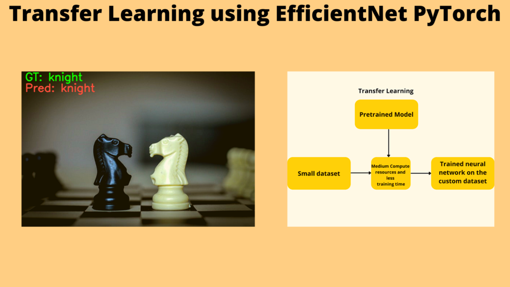
In this tutorial, we will use the EfficientNet model in PyTorch for transfer learning. We will carry out the transfer learning training on a small dataset in this tutorial. In the last tutorial, we went over image classification using pretrained EfficientNetB0 for image classification. Along with that, we also compared the forward pass time of the EfficientNetB0 model with that of ResNet50. If you are new to EfficinetNets, then the previous post may help you.

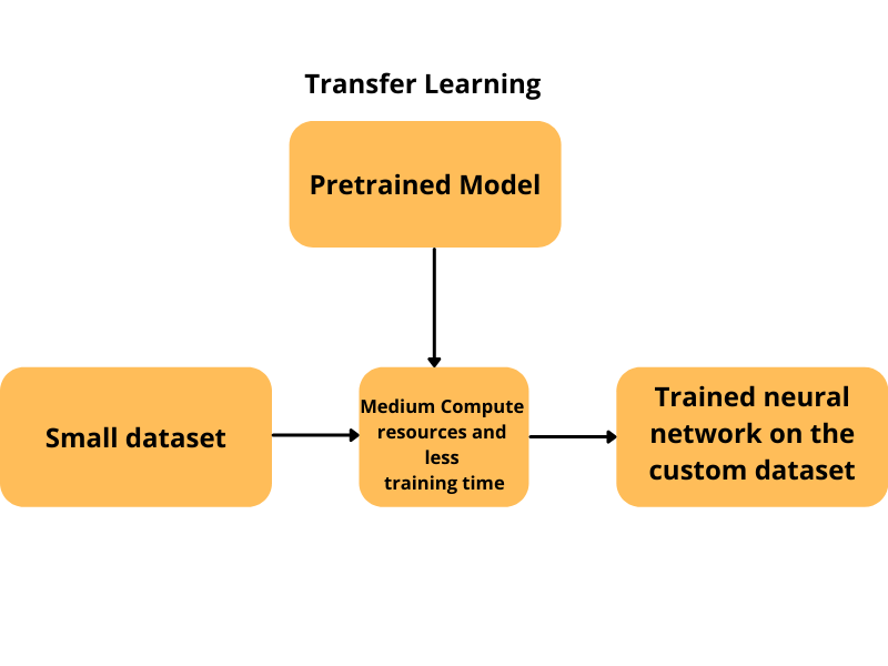
Here, we will take it one step further. The EfficientNet models are some of the best in deep learning and computer vision. They have already been trained on the ImageNet dataset. And there are a total of 8 such pretrained models in the EfficientNet family. And the power of these pretrained models actually shines when we have a small dataset to train on. In such situations, training from scratch does not really help much. But transfer learning can overcome those hurdles.

We will use one of those models in this tutorial for transfer learning using EfficientNet PyTorch. You will get to know all the details about the model and the dataset we will use as you move through the tutorial.

For now, let’s check out the points that we will cover in this tutorial.

• In this tutorial, we will choose a very small dataset to show the efficiency of transfer learning and fine-tuning using the EfficientNetB0 model.
• First, we will train the model from scratch without using pretrained weights.
• Then we will use the ImageNet pretrained weights and fine-tune the layers.
• Finally, we will check how the pretrained EfficientNetB0 model helps in achieving good results even when the training images are too small.

Now, let’s jump into the tutorial.

The Dataset

To show the efficiency of transfer learning in deep learning, it is always better to use a smaller dataset. Although the more data we have, the better. But in this case, as we will be showcasing transfer learning using EfficientNet PyTorch and how good the EfficientNetB0 model is, a relatively small dataset will be helpful.

Here, we will use the Chessman image dataset from Kaggle. This dataset contains only 556 images distributed over 6 classes. The following are the classes and the number of images in each class.

• Bishop: 87
• King: 76
• Knight: 106
• Pawn: 107
• Queen: 78
• Rook: 102

As you can see that dataset is a bit imbalanced. But the real worry is the extremely less number of images per class. And after splitting the dataset into a training and validation set, there will be even fewer images for the training. Looks like this dataset is going to be perfect for analyzing transfer learning using EfficientNet PyTorch.

The following figure shows one image from each class just to get an idea of the type of images we are dealing with here.

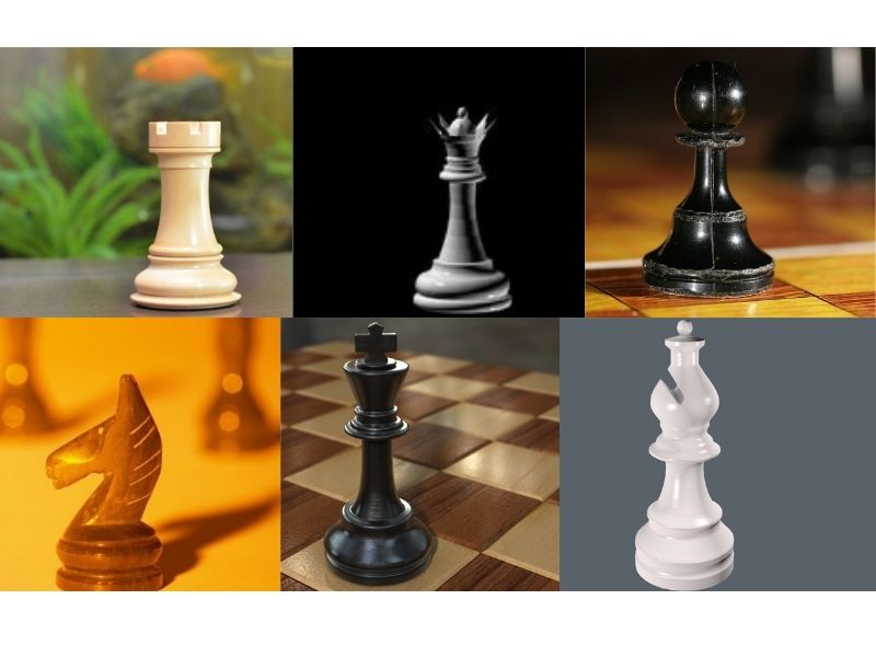
Before moving on to the next section, you may explore the dataset on your own a bit more here.

The Directory Structure

The following block shows the directory structure that we will use for this tutorial.

├── input
│   ├── Chessman-image-dataset
│   │   └── Chess
│   │       ├── Bishop [87 entries exceeds filelimit, not opening dir]
│   │       ├── King [76 entries exceeds filelimit, not opening dir]
│   │       ├── Knight [106 entries exceeds filelimit, not opening dir]
│   │       ├── Pawn [107 entries exceeds filelimit, not opening dir]
│   │       ├── Queen [78 entries exceeds filelimit, not opening dir]
│   │       └── Rook [102 entries exceeds filelimit, not opening dir]
│   └── test_images
├── outputs
│   ├── accuracy_pretrained_False.png
│   ├── accuracy_pretrained_True.png
│   ├── loss_pretrained_False.png
│   ├── loss_pretrained_True.png
│   ├── model_pretrained_False.pth
│   └── model_pretrained_True.pth
└── src
    ├── datasets.py
    ├── inference.py
    ├── model.py
    ├── train.py
    └── utils.py

Inside the parent project directory, there are three main directories.

• input: This contains the dataset in the Chessman-image-dataset folder. All the chess piece images are inside their respective class folders. This also contains the test_images folder containing the test images that we will use for inference after the training.
• outputs: We will use this folder to store all the training and validation graphs, and the trained models as well.
• src: This folder contains all the source code (five Python files). We will get into the coding details in a later section of the post.

If you download the zip file for this tutorial, you will get the entire directory structure already set up for you. As the dataset is small in size, you will also get the dataset with the downloaded file for this tutorial.

PyTorch Version

If you do not have PyTorch or have any version older than PyTorch 1.10, be sure to install/upgrade it. The EfficientNet models are available starting from PyTorch version 1.10 only.

With this, we are done with all the preliminary stuff. Let’s get into the coding part of the tutorial.

Transfer Learning using EfficientNet PyTorch

There are five Python files in this tutorial. For the training of the EfficientNetB0 model, we will need the following code files:

• utils.py
• datasets.py
• model.py
• train.py

After the training completes, we will write the code for inference in the inference.py script.

Note that all the code files will be present in the src folder.

The Helper Functions

We need a few helper functions. They are for saving the trained model and the accuracy and loss graphs. Let’s write the code for these in the utils.py file.

The following code block contains the import statements and the first function to save the trained models.

import torch
import matplotlib
import matplotlib.pyplot as plt

matplotlib.style.use('ggplot')


def save_model(epochs, model, optimizer, criterion, pretrained):
    """
    Function to save the trained model to disk.
    """
    torch.save({
                'epoch': epochs,
                'model_state_dict': model.state_dict(),
                'optimizer_state_dict': optimizer.state_dict(),
                'loss': criterion,
                }, f"../outputs/model_pretrained_{pretrained}.pth")

We need torch for saving the model and matplotlib for saving the accuracy and loss graphs.

The save_model() function accepts the number of epochs trained for, the model, the optimizer, loss function as parameters. The pretrained parameter is either True or False. We will use this in the name string while saving the model so that we can differentiate which model was trained with pretrained weights and which was not.

The above method of model saving will also allow us to resume training in the future if we want to do so.

Next is the function to save the loss and accuracy graphs.

def save_plots(train_acc, valid_acc, train_loss, valid_loss, pretrained):
    """
    Function to save the loss and accuracy plots to disk.
    """
    # accuracy plots
    plt.figure(figsize=(10, 7))
    plt.plot(
        train_acc, color='green', linestyle='-', 
        label='train accuracy'
    )
    plt.plot(
        valid_acc, color='blue', linestyle='-', 
        label='validataion accuracy'
    )
    plt.xlabel('Epochs')
    plt.ylabel('Accuracy')
    plt.legend()
    plt.savefig(f"../outputs/accuracy_pretrained_{pretrained}.png")
    
    # loss plots
    plt.figure(figsize=(10, 7))
    plt.plot(
        train_loss, color='orange', linestyle='-', 
        label='train loss'
    )
    plt.plot(
        valid_loss, color='red', linestyle='-', 
        label='validataion loss'
    )
    plt.xlabel('Epochs')
    plt.ylabel('Loss')
    plt.legend()
    plt.savefig(f"../outputs/loss_pretrained_{pretrained}.png")

The above save_plots() function also accepts the pretrained parameter so that graphs with different names are saved to disk for different sets of training runs.

Apart from that, it uses the general matplotlib methods to plot and save the graphs to disk.

Preparing the Dataset

Now, let’s prepare the datasets for the training.

We know that all the class folders are present in one directory and currently there is no training and validation split. So, we have to create the subsets on our own. Also, we will train twice. Once without pretrained weights and once with pretrained weights. In both cases, the image normalization, mean and standard deviation will be different. We need to take care of that too. Writing the code will make things clearer.

This code will go into the datasets.py file.

Starting with the import statements and a few required constants.

import torch

from torchvision import datasets, transforms
from torch.utils.data import DataLoader, Subset

# Required constants.
ROOT_DIR = '../input/Chessman-image-dataset/Chess'
VALID_SPLIT = 0.1
IMAGE_SIZE = 224 # Image size of resize when applying transforms.
BATCH_SIZE = 16 
NUM_WORKERS = 4 # Number of parallel processes for data preparation.

The constants define the data root directory path, the validation split ratio, the image size for resizing, the batch size, and the number of parallel processes for data preparation.

Training, Validation, and Normalization Transforms

Now, let’s define all the transforms that we need. This includes the training transforms/augmentations, validation transforms, and the image normalization transforms as well.

# Training transforms
def get_train_transform(IMAGE_SIZE, pretrained):
    train_transform = transforms.Compose([
        transforms.Resize((IMAGE_SIZE, IMAGE_SIZE)),
        transforms.RandomHorizontalFlip(p=0.5),
        transforms.GaussianBlur(kernel_size=(5, 9), sigma=(0.1, 5)),
        transforms.RandomAdjustSharpness(sharpness_factor=2, p=0.5),
        transforms.ToTensor(),
        normalize_transform(pretrained)
    ])
    return train_transform

# Validation transforms
def get_valid_transform(IMAGE_SIZE, pretrained):
    valid_transform = transforms.Compose([
        transforms.Resize((IMAGE_SIZE, IMAGE_SIZE)),
        transforms.ToTensor(),
        normalize_transform(pretrained)
    ])
    return valid_transform

# Image normalization transforms.
def normalize_transform(pretrained):
    if pretrained: # Normalization for pre-trained weights.
        normalize = transforms.Normalize(
            mean=[0.485, 0.456, 0.406],
            std=[0.229, 0.224, 0.225]
            )
    else: # Normalization when training from scratch.
        normalize = transforms.Normalize(
            mean=[0.5, 0.5, 0.5],
            std=[0.5, 0.5, 0.5]
        )
    return normalize

For the train_transform, we are applying random flipping, sharpness, and gaussian blurring as augmentations. We do not apply any augmentation to the validation set (valid_transform). But in both cases, we apply normalization transforms based on the pretrained parameter. If we are using EfficientNetB0 pretrained weights (when pretrained parameter is True), then the ImageNet normalization stats are applied from the normalize_transform() function.

Training/Validation Datasets and Data Loaders

The final part of the dataset preparation is preparing the training and validation datasets and data loaders. The following code block contains the functions which do that.

def get_datasets(pretrained):
    """
    Function to prepare the Datasets.

    :param pretrained: Boolean, True or False.

    Returns the training and validation datasets along 
    with the class names.
    """
    dataset = datasets.ImageFolder(
        ROOT_DIR, 
        transform=(get_train_transform(IMAGE_SIZE, pretrained))
    )
    dataset_test = datasets.ImageFolder(
        ROOT_DIR, 
        transform=(get_valid_transform(IMAGE_SIZE, pretrained))
    )
    dataset_size = len(dataset)

    # Calculate the validation dataset size.
    valid_size = int(VALID_SPLIT*dataset_size)
    # Radomize the data indices.
    indices = torch.randperm(len(dataset)).tolist()
    # Training and validation sets.
    dataset_train = Subset(dataset, indices[:-valid_size])
    dataset_valid = Subset(dataset_test, indices[-valid_size:])

    return dataset_train, dataset_valid, dataset.classes

def get_data_loaders(dataset_train, dataset_valid):
    """
    Prepares the training and validation data loaders.

    :param dataset_train: The training dataset.
    :param dataset_valid: The validation dataset.

    Returns the training and validation data loaders.
    """
    train_loader = DataLoader(
        dataset_train, batch_size=BATCH_SIZE, 
        shuffle=True, num_workers=NUM_WORKERS
    )
    valid_loader = DataLoader(
        dataset_valid, batch_size=BATCH_SIZE, 
        shuffle=False, num_workers=NUM_WORKERS
    )
    return train_loader, valid_loader 

The get_datasets() function accepts the pretrained parameter which it passes down to the get_train_transform() and get_valid_transform() functions. This is required for the image normalization transforms as we saw above. After that, we use the Subset class from PyTorch to create the training and validation splits for the datasets. This function returns the training & validation datasets along with the class names.

The get_data_loaders() function prepares the training and validation data loaders from the respective datasets and returns them.

This ends the dataset preparation part.

The EfficientNetB0 Model

The EfficientNetB0 is the smallest model in the EfficientNet family. With 1000 outputs classes (for ImageNet) in the final fully-connected layer, it has only 5.3 million parameters. This gives around 77.1% top-1 accuracy on the ImageNet dataset. Still, this beats ResNet50 which has 76.0% top-1 accuracy but with 26 million parameters.

Everything points towards the fact that EfficientNetB0 is a really good model. So, let’s start with this model in this tutorial.

Here, the code will go into the model.py file.

The following code block contains the entire function to build the model.

import torchvision.models as models
import torch.nn as nn

def build_model(pretrained=True, fine_tune=True, num_classes=10):
    if pretrained:
        print('[INFO]: Loading pre-trained weights')
    else:
        print('[INFO]: Not loading pre-trained weights')
    model = models.efficientnet_b0(pretrained=pretrained)

    if fine_tune:
        print('[INFO]: Fine-tuning all layers...')
        for params in model.parameters():
            params.requires_grad = True
    elif not fine_tune:
        print('[INFO]: Freezing hidden layers...')
        for params in model.parameters():
            params.requires_grad = False

    # Change the final classification head.
    model.classifier[1] = nn.Linear(in_features=1280, out_features=num_classes)
    return model

The build_model() function has the following parameters:

• pretrained: It will be a boolean value indicating whether we want to load the ImageNet weights or not.
• fine_tune: It is also a boolean value. When it is True, all the intermediate layers will also be trained.
• num_classes: Number of classes in the dataset.

We load the efficientnet_b0 model from the models module of torchvision on line 9. If you print the model, the last few layers will be the following:

EfficientNet(
  (features): Sequential(
    (0): ConvNormActivation(
      (0): Conv2d(3, 32, kernel_size=(3, 3), stride=(2, 2), padding=(1, 1), bias=False)
      (1): BatchNorm2d(32, eps=1e-05, momentum=0.1, affine=True, track_running_stats=True)
      (2): SiLU(inplace=True)
    )
...
...
...
  (classifier): Sequential(
    (0): Dropout(p=0.2, inplace=True)
    (1): Linear(in_features=1280, out_features=1000, bias=True)
  )
)

The above blocks shows the truncated structure of EfficientNetB0. The last block is the classifier block with the final layer being the fully-connected Linear layer with 1000 output features for the ImageNet dataset. But we have only 6 classes in our dataset. So, we need to change this layer here.

On line 21 of model.py, we modify only that layer so that the output features will match the number of classes in our dataset. The input features remain the same.

Other than that, we don’t add any additional Linear layers here. We keep everything else the same.

The Training Script

We have reached the final training script before we can start the training. This will be a bit long but easy to follow as we will just be connecting all the pieces completed till now.

We will write the training script in the train.py file.

Starting with the imports and building the argument parser.

import torch
import argparse
import torch.nn as nn
import torch.optim as optim
import time

from tqdm.auto import tqdm

from model import build_model
from datasets import get_datasets, get_data_loaders
from utils import save_model, save_plots

# construct the argument parser
parser = argparse.ArgumentParser()
parser.add_argument(
    '-e', '--epochs', type=int, default=20,
    help='Number of epochs to train our network for'
)
parser.add_argument(
    '-pt', '--pretrained', action='store_true',
    help='Whether to use pretrained weights or not'
)
parser.add_argument(
    '-lr', '--learning-rate', type=float,
    dest='learning_rate', default=0.0001,
    help='Learning rate for training the model'
)
args = vars(parser.parse_args())

From lines 9 to 11, we import all our custom modules. For the argument parser, we have the following flags:

• --epochs: The number of epochs to train for.
• --pretrained: Whenever we pass this flag from the command line, pretrained EfficientNetB0 weights will be loaded.
• --learning-rate: The learning rate for training. As you might remember, we will train twice, once with pretrained weights, once without. Both cases require different learning rates, so, it is better to control it while executing the training script.

The Training and Validation Functions

The training function is going to be simple and like any other image classification function in PyTorch.

# Training function.
def train(model, trainloader, optimizer, criterion):
    model.train()
    print('Training')
    train_running_loss = 0.0
    train_running_correct = 0
    counter = 0
    for i, data in tqdm(enumerate(trainloader), total=len(trainloader)):
        counter += 1
        image, labels = data
        image = image.to(device)
        labels = labels.to(device)
        optimizer.zero_grad()
        # Forward pass.
        outputs = model(image)
        # Calculate the loss.
        loss = criterion(outputs, labels)
        train_running_loss += loss.item()
        # Calculate the accuracy.
        _, preds = torch.max(outputs.data, 1)
        train_running_correct += (preds == labels).sum().item()
        # Backpropagation
        loss.backward()
        # Update the weights.
        optimizer.step()
    
    # Loss and accuracy for the complete epoch.
    epoch_loss = train_running_loss / counter
    epoch_acc = 100. * (train_running_correct / len(trainloader.dataset))
    return epoch_loss, epoch_acc

We pass the image batches through the model, calculate the loss, do backpropagation, and update the model weights. Finally, we return the epoch-wise loss and accuracy.

The validation function is almost the same. Except, we don’t need backpropagation and model weight update here.

# Validation function.
def validate(model, testloader, criterion):
    model.eval()
    print('Validation')
    valid_running_loss = 0.0
    valid_running_correct = 0
    counter = 0
    with torch.no_grad():
        for i, data in tqdm(enumerate(testloader), total=len(testloader)):
            counter += 1
            
            image, labels = data
            image = image.to(device)
            labels = labels.to(device)
            # Forward pass.
            outputs = model(image)
            # Calculate the loss.
            loss = criterion(outputs, labels)
            valid_running_loss += loss.item()
            # Calculate the accuracy.
            _, preds = torch.max(outputs.data, 1)
            valid_running_correct += (preds == labels).sum().item()
        
    # Loss and accuracy for the complete epoch.
    epoch_loss = valid_running_loss / counter
    epoch_acc = 100. * (valid_running_correct / len(testloader.dataset))
    return epoch_loss, epoch_acc

The Main Code Block

The main code block will encompass everything above, start the training, plot the graphs, and save the models to disk.

if __name__ == '__main__':
    # Load the training and validation datasets.
    dataset_train, dataset_valid, dataset_classes = get_datasets(args['pretrained'])
    print(f"[INFO]: Number of training images: {len(dataset_train)}")
    print(f"[INFO]: Number of validation images: {len(dataset_valid)}")
    print(f"[INFO]: Class names: {dataset_classes}\n")
    # Load the training and validation data loaders.
    train_loader, valid_loader = get_data_loaders(dataset_train, dataset_valid)

    # Learning_parameters. 
    lr = args['learning_rate']
    epochs = args['epochs']
    device = ('cuda' if torch.cuda.is_available() else 'cpu')
    print(f"Computation device: {device}")
    print(f"Learning rate: {lr}")
    print(f"Epochs to train for: {epochs}\n")

    model = build_model(
        pretrained=args['pretrained'], 
        fine_tune=True, 
        num_classes=len(dataset_classes)
    ).to(device)
    
    # Total parameters and trainable parameters.
    total_params = sum(p.numel() for p in model.parameters())
    print(f"{total_params:,} total parameters.")
    total_trainable_params = sum(
        p.numel() for p in model.parameters() if p.requires_grad)
    print(f"{total_trainable_params:,} training parameters.")

    # Optimizer.
    optimizer = optim.Adam(model.parameters(), lr=lr)
    # Loss function.
    criterion = nn.CrossEntropyLoss()

    # Lists to keep track of losses and accuracies.
    train_loss, valid_loss = [], []
    train_acc, valid_acc = [], []
    # Start the training.
    for epoch in range(epochs):
        print(f"[INFO]: Epoch {epoch+1} of {epochs}")
        train_epoch_loss, train_epoch_acc = train(model, train_loader, 
                                                optimizer, criterion)
        valid_epoch_loss, valid_epoch_acc = validate(model, valid_loader,  
                                                    criterion)
        train_loss.append(train_epoch_loss)
        valid_loss.append(valid_epoch_loss)
        train_acc.append(train_epoch_acc)
        valid_acc.append(valid_epoch_acc)
        print(f"Training loss: {train_epoch_loss:.3f}, training acc: {train_epoch_acc:.3f}")
        print(f"Validation loss: {valid_epoch_loss:.3f}, validation acc: {valid_epoch_acc:.3f}")
        print('-'*50)
        time.sleep(5)
        
    # Save the trained model weights.
    save_model(epochs, model, optimizer, criterion, args['pretrained'])
    # Save the loss and accuracy plots.
    save_plots(train_acc, valid_acc, train_loss, valid_loss, args['pretrained'])
    print('TRAINING COMPLETE')

The above code block is almost entirely self-explanatory. Still, going through some of the import parts.

• Starting from line 103, we load the EfficientNetB0 model. We pass the --pretrained flag to control whether to load to ImageNet weights or not. But in both cases we will train all the layers of the network. This is because it is unlikely that the model would have seen such chess piece images in the ImageNet dataset. It might have, still, it is better to tune the model weights with the specific dataset when we have such a small dataset.
• The optimizer is Adam, with the learning rate being controlled by the --learning-rate flag.
• We are using CrossEntropyLoss as there are multiple classes here.
• From line 125, we start the training of model for the number of epochs as specified while executing the script.

After the training completes, we just save the accuracy and loss graphs to disk along with the trained model. Note that the graph and model names’ strings contain the args['pretrained'] flag/variable so that we can differentiate between them later on.

Executing train.py

Now, it’s time to execute our training script. As discussed earlier, we will run the training twice. Once without pretrained weights, and again with.

Execute the following commands in your terminal/command line within the src directory.

Starting the training without pretrained weights.

python train.py --epochs 50 --learning-rate 0.001

As we are not loading the pretrained weights, we are using 0.001 as the learning rate. Any value less than this might be too slow to train or may not train at all. The following block contains the truncated results from the terminal.

[INFO]: Number of training images: 497
[INFO]: Number of validation images: 55
[INFO]: Class names: ['Bishop', 'King', 'Knight', 'Pawn', 'Queen', 'Rook']

Computation device: cuda
Learning rate: 0.001
Epochs to train for: 50

[INFO]: Not loading pre-trained weights
[INFO]: Fine-tuning all layers...
4,015,234 total parameters.
4,015,234 training parameters.
[INFO]: Epoch 1 of 50
Training
100%|████████████████████████████████████████████████████████████████████| 32/32 [00:02<00:00, 11.62it/s]
Validation
100%|██████████████████████████████████████████████████████████████████████| 4/4 [00:00<00:00,  6.19it/s]
Training loss: 1.974, training acc: 12.475
Validation loss: 1.756, validation acc: 18.182
--------------------------------------------------
...
[INFO]: Epoch 50 of 50
Training
100%|████████████████████████████████████████████████████████████████████| 32/32 [00:02<00:00, 14.89it/s]
Validation
100%|██████████████████████████████████████████████████████████████████████| 4/4 [00:00<00:00,  6.05it/s]
Training loss: 0.531, training acc: 83.501
Validation loss: 1.153, validation acc: 61.818
--------------------------------------------------
TRAINING COMPLETE

As you monitor the training, you might see that the validation accuracy was fluctuating a lot. In the last epoch, we have 61.818% validation accuracy and 1.153 validation loss.

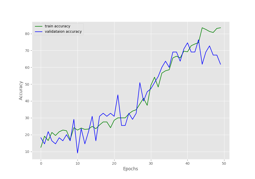
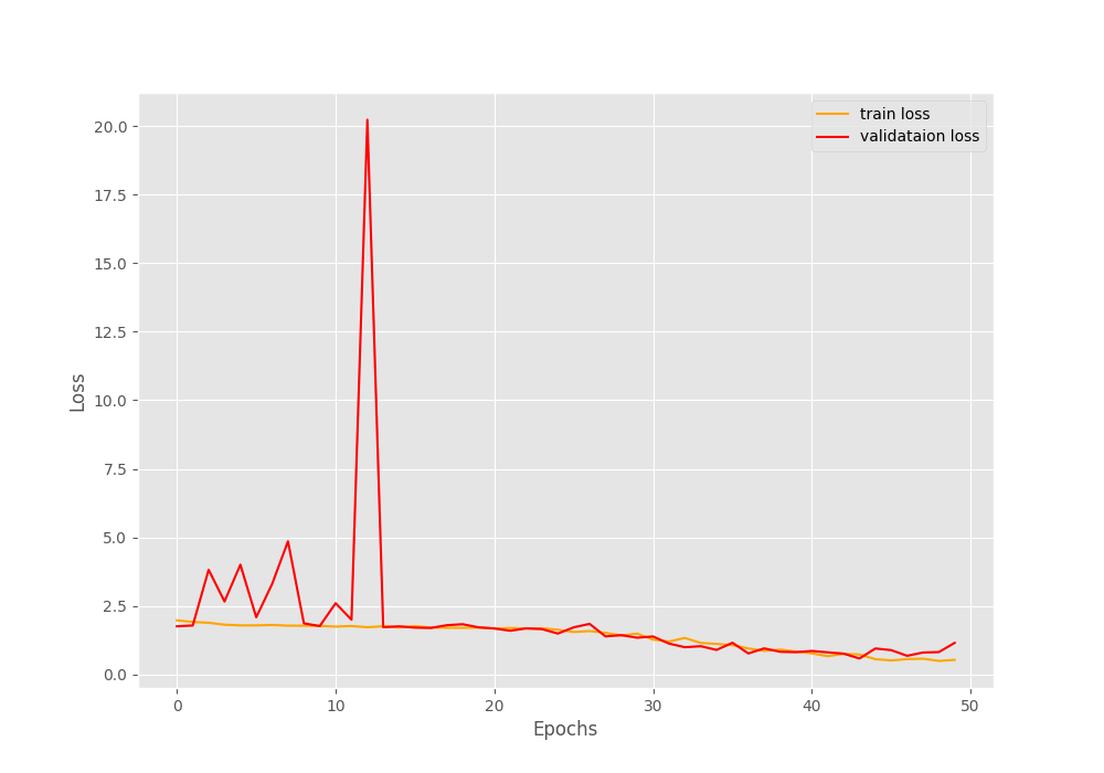
From the above loss and accuracy graphs, it is clearly visible that the model was starting to overfit after around 45 epochs. Although the trained model has been saved to disk, the results are not good enough to run an inference for sure.

Therefore, now, let’s train with pretrianed weights. This time, let’s use a learning rate of 0.0001 so that we do not update the pretrained weights suddenly.

python train.py --pretrained --epochs 50 --learning-rate 0.0001

The following are the outputs.

[INFO]: Number of training images: 497
[INFO]: Number of validation images: 55
[INFO]: Class names: ['Bishop', 'King', 'Knight', 'Pawn', 'Queen', 'Rook']

Computation device: cuda
Learning rate: 0.0001
Epochs to train for: 50

[INFO]: Loading pre-trained weights
[INFO]: Fine-tuning all layers...
4,015,234 total parameters.
4,015,234 training parameters.
[INFO]: Epoch 1 of 50
Training
100%|████████████████████████████████████████████████████████████████████| 32/32 [00:03<00:00,  9.66it/s]
Validation
100%|██████████████████████████████████████████████████████████████████████| 4/4 [00:00<00:00,  7.18it/s]
Training loss: 1.733, training acc: 28.773
Validation loss: 1.660, validation acc: 40.000
--------------------------------------------------
--------------------------------------------------
[INFO]: Epoch 50 of 50
Training
100%|████████████████████████████████████████████████████████████████████| 32/32 [00:02<00:00, 15.69it/s]
Validation
100%|██████████████████████████████████████████████████████████████████████| 4/4 [00:00<00:00,  7.49it/s]
Training loss: 0.060, training acc: 99.598
Validation loss: 0.098, validation acc: 98.182
--------------------------------------------------
TRAINING COMPLETE

This time also you will see fluctuation in the validation metrics. But the final epoch’s validation results are much better. We have validation accuracy of more than 98% and validation loss of 0.098.

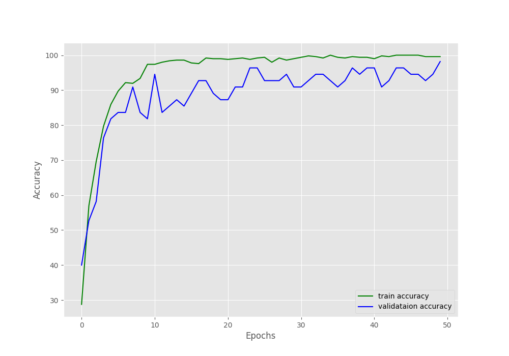
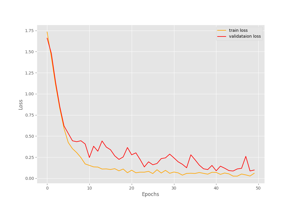
The accuracy and loss graphs seem to be increasing and decreasing respectively till the end of training. So, that’s a good sign. Looks like the pretrained weights really helped a lot. There is a huge difference compared to the previous results even though we have only 556 images.

Hopefully, this time, the model has learned enough to correctly predict unseen chess piece images. We will only get to know this after we run the inference.

The Inference Script

Here, we will write the code to run inference using the trained model. All the test images are inside the input/test_images directory.

The inference code will go into the inference.py script.

import torch
import cv2
import numpy as np
import glob as glob
import os

from model import build_model
from torchvision import transforms

# Constants.
DATA_PATH = '../input/test_images'
IMAGE_SIZE = 224
DEVICE = 'cpu'

# Class names.
class_names = ['Bishop', 'King', 'Knight', 'Pawn', 'Queen', 'Rook']

# Load the trained model.
model = build_model(pretrained=False, fine_tune=False, num_classes=6)
checkpoint = torch.load('../outputs/model_pretrained_True.pth', map_location=DEVICE)
print('Loading trained model weights...')
model.load_state_dict(checkpoint['model_state_dict'])

We start with the imports and define the required constants. We also define a list containing the class names which we will use while visualizing the outputs.

Then we load the trained weights from the model checkpoint saved from training and fine-tuning the pretrained EfficientNetB0 model.

The next code block iterates over all the test images and runs the inference on each one of them.

# Get all the test image paths.
all_image_paths = glob.glob(f"{DATA_PATH}/*")
# Iterate over all the images and do forward pass.
for image_path in all_image_paths:
    # Get the ground truth class name from the image path.
    gt_class_name = image_path.split(os.path.sep)[-1].split('.')[0]
    # Read the image and create a copy.
    image = cv2.imread(image_path)
    orig_image = image.copy()
    
    # Preprocess the image
    image = cv2.cvtColor(image, cv2.COLOR_BGR2RGB)
    transform = transforms.Compose([
        transforms.ToPILImage(),
        transforms.Resize((IMAGE_SIZE, IMAGE_SIZE)),
        transforms.ToTensor(),
        transforms.Normalize(
            mean=[0.485, 0.456, 0.406],
            std=[0.229, 0.224, 0.225]
        )
    ])
    image = transform(image)
    image = torch.unsqueeze(image, 0)
    image = image.to(DEVICE)
    
    # Forward pass throught the image.
    outputs = model(image)
    outputs = outputs.detach().numpy()
    pred_class_name = class_names[np.argmax(outputs[0])]
    print(f"GT: {gt_class_name}, Pred: {pred_class_name.lower()}")
    # Annotate the image with ground truth.
    cv2.putText(
        orig_image, f"GT: {gt_class_name}",
        (10, 25), cv2.FONT_HERSHEY_SIMPLEX,
        1.0, (0, 255, 0), 2, lineType=cv2.LINE_AA
    )
    # Annotate the image with prediction.
    cv2.putText(
        orig_image, f"Pred: {pred_class_name.lower()}",
        (10, 55), cv2.FONT_HERSHEY_SIMPLEX,
        1.0, (100, 100, 225), 2, lineType=cv2.LINE_AA
    ) 
    cv2.imshow('Result', orig_image)
    cv2.waitKey(0)
    cv2.imwrite(f"../outputs/{gt_class_name}.png", orig_image)

We iterate over all the paths, read the image and also apply the required preprocessing transforms. The forward pass happens on line 49. The next few lines of code annotate the original image with the ground truth and predicted class name. Along with that, we visualize the result and also save it to disk.

This is a very simple set of code for inference as we are only dealing with images here.

Execute inference.py Script

This is the last part of transfer learning with EfficientNet PyTorch. We will run the inference on new unseen images, and hopefully, the trained model will be able to correctly classify most of the images. There is one image from each class.

python inference.py 

You will also see the output on the terminal screen. Let’s take a look at the results that are saved to disk.

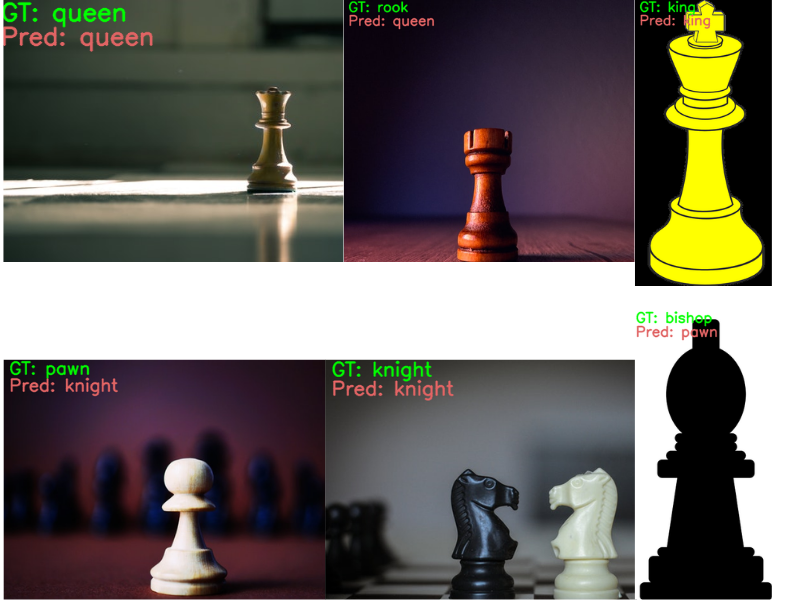
The model was able to correctly predict the King, Queen, and Knight. The other three classes’ predictions are wrong. This might seem like a bad performance. But if you think about it, the model was able to learn this from just around 500 images. With a bit more appropriate augmentation applied and a few more epochs of training, the model might be able to classify all of these correctly. Also, trying out a larger EfficientNet model like EfficientNetB1 may also help.

Summary and Conclusion

In this tutorial, you learned how transfer learning using the EfficientNet PyTorch model can give good results even when we have very little training data. We carried the experiment on a set of chess piece images. Without transfer learning, the results were not so good. But with transfer learning and fine-tuning, we were able or improve the classification accuracy quite a lot. I hope that you learned something new from this tutorial.

If you have any doubts, thoughts, or suggestions, please leave them in the comment section. I will surely address them.

You can contact me using the Contact section. You can also find me on LinkedIn, and Twitter.