PlantDoc Dataset for Plant Disease Recognition using PyTorch

Recognizing diseases of plants in their natural habitat is a tough task. When training a deep learning model, the image will contain objects in the background most of the time. These may include other parts of the plant, the ground, or even the hands of the person who is taking the photograph. Of course, we want the model to focus on the plant of interest only. But for that, we need the training dataset to resemble real-world scenarios, so that the model can learn those features. PlantDoc is one such dataset. In this post, we will use the PlantDoc dataset for plant disease recognition. We will use the PyTorch deep learning library for this.

Plant disease recognition using the PlantDoc dataset can be very challenging. Especially when not using very large networks. For that reason, we will train three different neural networks in this post and analyze which one performs the best.

We will cover the following topics in this tutorial:

• We will start with the exploration of the PlantDoc dataset. Here, we will also discuss why datasets like PlantDoc are important.
• Next, we will discuss the three models that we will fine-tune for the PlantDoc dataset for disease recognition.
• Then we will check the directory structure of the project.
• After that, we will discuss some of the important parts of the code. This includes model preparation and dataset preparation.
• Then we will train the model, discuss the results, and test them on a held-out split of the PlantDoc dataset.
• Finally, we will run inference on some unseen images using the model which performs best on the test set.

Let’s get into the technical details without any further delay.

The PlantDoc Dataset for Plant Disease Recognition

The PlantDoc dataset is a collection of images for visual plant disease recognition and detection. It has annotations for both, plant disease recognition and plant disease detection. But in this blog post, we will focus on plant disease recognition.

PlantDoc-Dataset is the official GitHub repository containing the dataset for plant disease recognition. But we will use this Kaggle PlantDoc dataset. The only reason is that the image names have been cleaned which prevents certain path errors on the Windows OS.

The dataset also has an accompanying paper on arxiv. You may give the paper a read to get additional details. This includes the dataset collection method, the filtering method, and also benchmarks and results according to the author’s experiments.

The final PlantDoc dataset contains 2,598 images and 27 classes. These 27 classes include different diseases belonging to the same plants as well. In fact, there are 13 plant species, and 17 classes of diseases in the dataset.

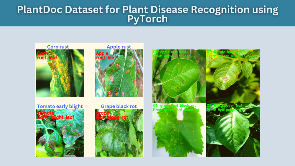
Here, are a few images from the dataset.

We can see the variety in the background in the PlantDoc dataset. This will surely help deep learning models to learn the surrounding context.

The dataset already comes with a train test split. Each class in the test split contains around 8-12 images. The classes in the train split contain as low 54 images and go up to 137 images in some of the classes.

For now, you may go ahead and download the dataset from Kaggle.

Why is the PlantDoc Dataset for Plant Disease Recognition Important?

In the previous tutorial, we covered plant disease recognition using the PlantVillage dataset. That dataset contains much more images (more than 50000) compared to the PlantDoc dataset.

But if you remember, even if we were getting high test accuracy, the inference results on the real-world images showed otherwise. The PlantiVillage dataset contains images taken in a controlled environment with a static background. But the real-world images will definitely contain different types of backgrounds.

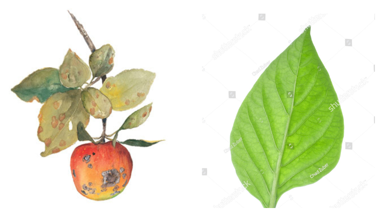
For example, take a look at the following image.

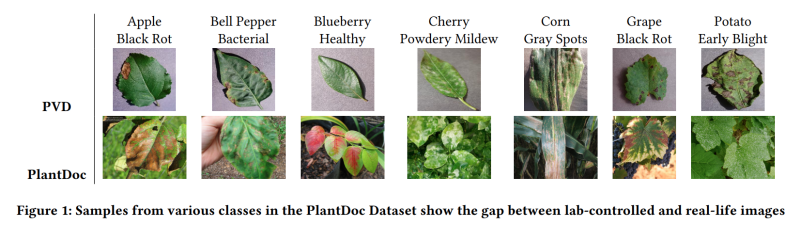
The above figure clearly shows the difference between the images of the PlantDoc and PlantVillage datasets. The extra background information is essential for the model to see during the training if we want it to perform well on real-world images.

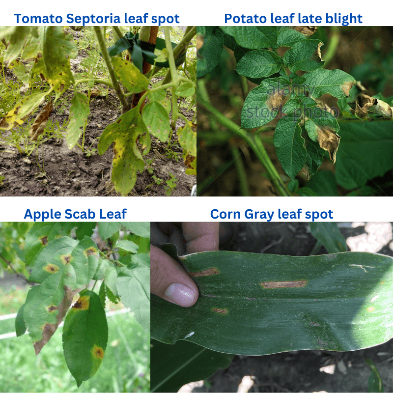
Still, if we go through all images from the PlantDoc dataset, we can find a few images with similar white backgrounds, such as the following.

These images have been collected from the internet, and some images are bound to contain such backgrounds. But we will focus on training three different convolutional neural networks in this post. And check the inference results on some of the same images that we did in the case of PlantVillage experiment.

Training Experiments to Carry Out for PlantDoc Plant Disease Recognition

For the training experiments, we choose three models. They are:

• EfficientNetB0: In the previous tutorial where we trained models on the PlantVillage dataset, the EfficientNetB0 model performed the best. So, the results from training the EfficientNetB0 model will form the baseline.
• ResNet18: The PlantDoc dataset is a considerably difficult dataset compared to the PlantVillage dataset. So, next we will move on to larger models like ResNets. First, we will train the ResNet18 model.
• ResNet50: The next residual neural network that we will train is the ResNet50 model. It is much larger than both, EfficientNetB0 and ResNet18, and should give much better results.

Directory Structure

As we are going to carry out three different training experiments for this blog post, let’s discuss how we are going to structure it.

.
├── input
│   ├── inference_data
│   │   ├── apple_rust.png
│   │   ...
│   │   └── tomato_early_blight.jpg
│   |── PlantDoc-Dataset
│       ├── test
│       │   ├── Apple leaf
│       │   ...
│       │   ├── Tomato mold leaf
│       │   └── Tomato Septoria leaf spot
│       └── train
│           ├── Apple leaf
│           ...
│           └── Tomato Septoria leaf spot
├── outputs
│   ├── efficientnetb0
│   │   ├── accuracy.png
│   │   ├── best_model.pth
│   │   ├── loss.png
│   │   └── model.pth
│   ├── inference_results
│   │   ├── efficientnetb0
│   │      ...
│   ├── resnet18
│   │   ├── accuracy.png
│   │   ├── best_model.pth
│   │   ├── loss.png
│   │   └── model.pth
│   ├── resnet50
│   │   ├── accuracy.png
│   │   ├── best_model.pth
│   │   ├── loss.png
│   │   └── model.pth
│   └── test_results
│       ├── efficientnetb0
│       │   ...
│       ├── resnet18
│       │   ...
│       └── resnet50
│           ...
└── src
    ├── class_names.py
    ├── datasets.py
    ├── inference.py
    ├── model.py
    ├── test.py
    ├── train.py
    └── utils.py

75 directories, 747 files

• The input directory contains all the data related files. After extracting the PlantDoc dataset, we get the PlantDoc-Dataset directory. This contains the train and test subdirectories with folder names same as class names holding the images. Next, the inferene_data directory contains a few images from the internet that we will use for inference after training, testing, and validation.
• Then we have the outputs directory with all the training, testing, and inference related outputs. All the subdirectories with model names contains the training outputs. Simiarly, all the test_results and inference_results directories contains folders with model names to seggregate the outputs of each model.
• Finally, we have the src directory containing all the Python code files. There are seven Python files. But we will discuss only the important parts of the code. Still, all the code files will be available for download.

PyTorch Version

The code for this project was developed using PyTorch 1.13.0. PyTorch 1.12.0 and 1.12.1 should also work. But other lower versions will not work as the code uses the latest API to load either the ImageNet1KV1 or ImageNet1KV2 pretrained weights of the models. In case you need to, you can get the installation commands of PyTorch from here.

All the code files along with the appropriate directory structure are available for download. You just need to keep the dataset in the correct structure as shown above if you wish to run the code locally.

Using PyTorch for PlantDoc Plant Disease Recognition

Let’s jump into the coding and training aspects of the post now.

The PlantDoc Dataset Class Names

As discussed earlier, there are 27 classes in the PlantDoc dataset. Let’s create a separate class_names.py containing all the class names in a list. Then, we can import that list whenever we want to use it in another file.

Download Code

class_names = [
    'Apple Scab Leaf', 'Apple leaf', 'Apple rust leaf', 'Bell_pepper leaf', 
    'Bell_pepper leaf spot', 'Blueberry leaf', 'Cherry leaf', 'Corn Gray leaf spot', 
    'Corn leaf blight', 'Corn rust leaf', 'Peach leaf', 'Potato leaf early blight', 
    'Potato leaf late blight', 'Raspberry leaf', 'Soyabean leaf',
    'Squash Powdery mildew leaf', 'Strawberry leaf', 'Tomato Early blight leaf', 
    'Tomato Septoria leaf spot', 'Tomato leaf', 'Tomato leaf bacterial spot', 
    'Tomato leaf late blight', 'Tomato leaf mosaic virus', 
    'Tomato leaf yellow virus', 'Tomato mold leaf', 'grape leaf', 'grape leaf black rot'
    ]

Note: All those classes that only contain the name of the plant or fruit followed by leaf indicate images belonging to healthy leaves. For example, grape leaf indicates that the images for this class contains healthy leaves of the grape plant.

Helper Function and Utilities

We will need some helper functions and utility classes to make the training process easier. For that, we use the utils.py file.

This file contains:

• The SaveBestModel class to save the best model based on the least validation loss.
• The save_model function to save the model after the training completes.
• And the save_plots function to save the loss and accuracy graphs.

It is worthwhile to note that, the save_model function saves the optimizer state dictionary as well. This is helpful in case we want to resume training later.

Preparing the Datasets and Data Loaders

The next important part is creating the datasets and the data loaders. Although the process is quite simple, let’s focus on a few things.

First of all, there is already a train and a test split available in the dataset. But we will keep the test split aside for now and divide the training split into a train and a validation set. After training, we will use the test split that comes with the dataset for testing the trained models.

The dataset preparation code resides in the datasets.py file.

We are applying quite a few image augmentation techniques from torchvision which help the models from overfitting too quickly. They are:

• RandomHorizontalFlip
• RandomVerticalFlip
• RandomRotation
• ColorJitter
• GaussianBlur
• RandomAdjustSharpness

Along with that, we also apply the ImageNet mean and standard deviation values for the normalization. This is for both, the training and validation set.

Further, some other important points to factor here:

• We are resizing all images to 224×224 resolution. Higher resolution images will give better results but also take longer to train.
• By default, the number of parallel workers for the data loader is 4.
• We are using 15% of the training split (that comes with the dataset) for validation and the rest for training.

The above are a few things we need to keep in mind about the dataset preparation.

Preparing the Neural Network Models for PlantDoc Plant Disease Recognition

As discussed earlier, we will be training three different models. For that, we will need to write the model creation code a bit differently.

The model preparation code goes into the model.py file. Let’s check out its entire content.

from torchvision import models

import torch.nn as nn

def model_config(model_name='resnet18'):
    model = {
        'efficientnetb0': models.efficientnet_b0(weights='DEFAULT'),
        'resnet18': models.resnet18(weights='DEFAULT'),
        'resnet50': models.resnet50(weights='DEFAULT')
    }
    return model[model_name]

def build_model(model_name='efficientnetb0', fine_tune=True, num_classes=10):
    model = model_config(model_name)
    if fine_tune:
        print('[INFO]: Fine-tuning all layers...')
        for params in model.parameters():
            params.requires_grad = True
    if not fine_tune:
        print('[INFO]: Freezing hidden layers...')
        for params in model.parameters():
            params.requires_grad = False

    if model_name == 'efficientnetb0':
        model.classifier[1] = nn. Linear(in_features=1280, out_features=num_classes)
    if model_name == 'resnet18':
        model.fc = nn.Linear(in_features=512, out_features=num_classes)
    if model_name == 'resnet50':
        model.fc = nn.Linear(in_features=2048, out_features=num_classes)
    return model

We have a model_config function that contains a model dictionary. The keys are strings indicating model names that match with the models module from torchvision. Whatever model name we pass to the function, the function will return that model along with the pretrained weights.

In the build_model function, we create the final classification layer of each model. For that, we use a few simple if statements. Note that we can also control whether we want to fine tune the hidden layers or not based on the fine_tune parameter.

The Training Script

All the training code is available in the train.py script. This is the executable driver script that combines all the code that we discussed above.

The following are the command line argument flags that we can pass while executing the train.py script.

• --epochs: The number of epochs we want to train for.
• --learning-rate: The learning rate for the optimizer. It is 0.001 by default.
• --model: The model name string. We can pass one of efficientnetb0, resnet18, resnet50.
• --batch-size: Batch size for the data loaders. It is 32 by default.
• --fine-tune: It is a boolean argument and passing this will make all the parameters of the model trainable.

Other than that, we will be using the SGD optimizer with momentum. The default learning rate is 0.001 as we are using the pretrained weights.

Training the Models for PlantDoc Plant Disease Recognition

Let’s run all the training experiments for the PlantDoc Plant Disease Recognition now. We will train each model and analyze the results.

We will be training all the models for 30 epochs.

All the training, testing, and inference experiments were carried out on a laptop with:

• 6 GB GTX 1060 GPU
• 16 GB DDR4 RAM
• i7 8th generation CPU

Training EfficientNetB0 on the PlantDoc Dataset

To train the EfficientNetB0 model, simply execute the following command in the terminal within the src directory.

python train.py --model efficientnetb0 --epochs 30 --fine-tune

The following are the sample outputs from the terminal.

[INFO]: Number of training images: 1969
[INFO]: Number of validation images: 347
[INFO]: Classes: ['Apple Scab Leaf', 'Apple leaf', 'Apple rust leaf', 'Bell_pepper leaf', 'Bell_pepper leaf spot', 'Blueberry leaf', 'Cherry leaf', 'Corn Gray leaf spot', 'Corn leaf blight', 'Corn rust leaf', 'Peach leaf', 'Potato leaf early blight', 'Potato leaf late blight', 'Raspberry leaf', 'Soyabean leaf', 'Squash Powdery mildew leaf', 'Strawberry leaf', 'Tomato Early blight leaf', 'Tomato Septoria leaf spot', 'Tomato leaf', 'Tomato leaf bacterial spot', 'Tomato leaf late blight', 'Tomato leaf mosaic virus', 'Tomato leaf yellow virus', 'Tomato mold leaf', 'grape leaf', 'grape leaf black rot']
Computation device: cuda
Learning rate: 0.001
Epochs to train for: 30

[INFO]: Fine-tuning all layers...
.
.
.
[INFO]: Epoch 1 of 30
Training
100%|███████████████████████████████████████████████| 62/62 [00:29<00:00,  2.07it/s]
Validation
100%|███████████████████████████████████████████████| 11/11 [00:04<00:00,  2.63it/s]
Training loss: 3.221, training acc: 10.157
Validation loss: 3.022, validation acc: 22.767

Best validation loss: 3.021585312756625

Saving best model for epoch: 1

--------------------------------------------------
.
.
.
[INFO]: Epoch 30 of 30
Training
100%|███████████████████████████████████████████████| 62/62 [00:29<00:00,  2.13it/s]
Validation
100%|███████████████████████████████████████████████| 11/11 [00:03<00:00,  2.83it/s]
Training loss: 0.593, training acc: 82.631
Validation loss: 1.067, validation acc: 68.012
--------------------------------------------------
TRAINING COMPLETE

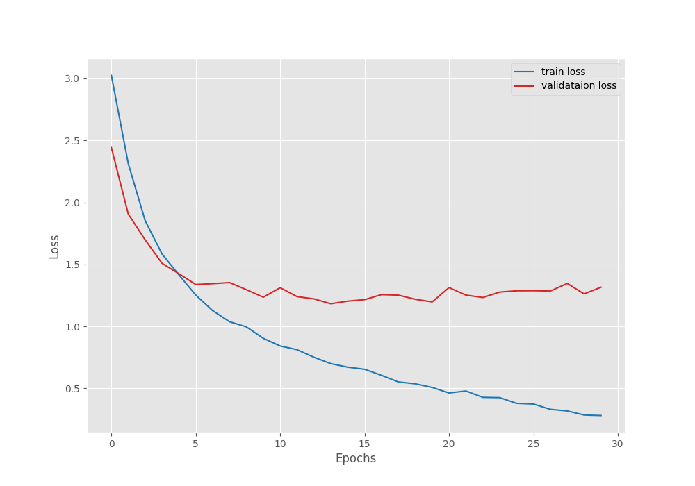
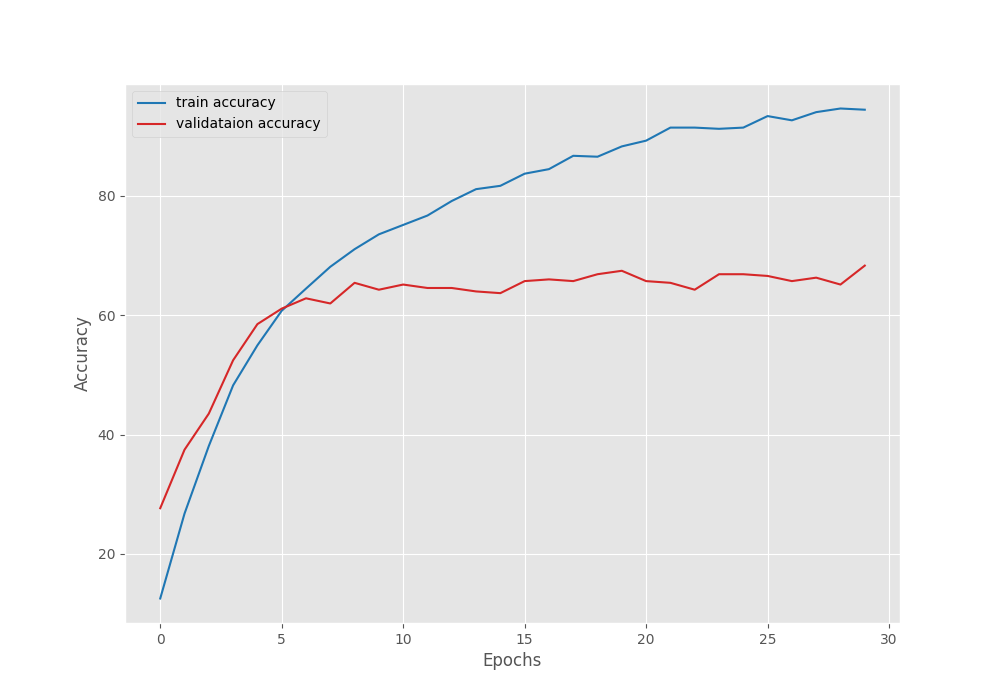
The best model for EfficientNetB0 training was saved on epoch 28. For that epoch, the validation loss was 1.048 and the validation accuracy was 68.87%.

The following are the accuracy and loss graphs for the training.

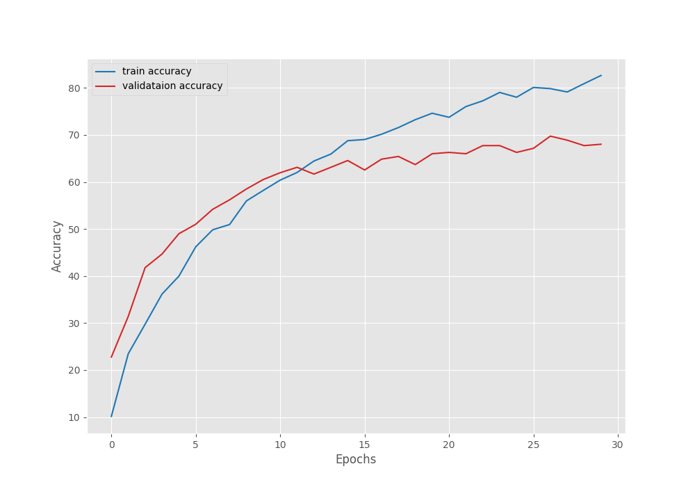
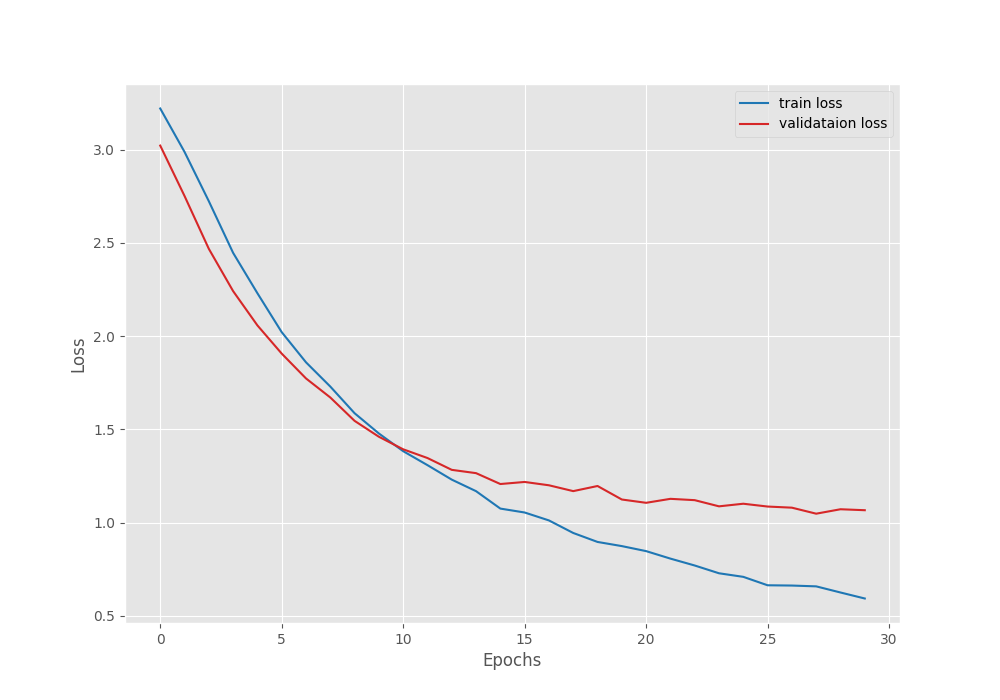
It’s pretty clear that we can train the model for longer. The loss and accuracy were still improving till the end of training.

Training ResNet18 on the PlantDoc Dataset

Now, let’s train the ResNet18 model. We just need to change the --model flag.

python train.py --model resnet18 --epochs 30 --fine-tune

Here are the outputs.

[INFO]: Epoch 1 of 30
Training
100%|███████████████████████████████████████████████| 62/62 [00:28<00:00,  2.15it/s]
Validation
100%|███████████████████████████████████████████████| 11/11 [00:03<00:00,  2.98it/s]
Training loss: 3.025, training acc: 16.150
Validation loss: 2.442, validation acc: 38.905

Best validation loss: 2.4424689683047207

Saving best model for epoch: 1

--------------------------------------------------
.
.
.
[INFO]: Epoch 29 of 30
Training
100%|███████████████████████████████████████████████| 62/62 [00:25<00:00,  2.40it/s]
Validation
100%|███████████████████████████████████████████████| 11/11 [00:03<00:00,  3.23it/s]
Training loss: 0.285, training acc: 92.280
Validation loss: 1.262, validation acc: 63.112
--------------------------------------------------
[INFO]: Epoch 30 of 30
Training
100%|███████████████████████████████████████████████| 62/62 [00:25<00:00,  2.41it/s]
Validation
100%|███████████████████████████████████████████████| 11/11 [00:03<00:00,  3.23it/s]
Training loss: 0.281, training acc: 92.280
Validation loss: 1.316, validation acc: 59.942
--------------------------------------------------
TRAINING COMPLETE

The best model for ResNet18 was saved after epoch 14 where the validation accuracy was 61.96%. After that, the model started to overfit a bit. We can confirm this from the following graphs.

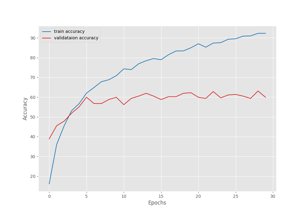
As you can see, the loss values are increasing slightly after epoch 14.

Another important point to note here is that the best validation accuracy is lower compared to that of EffcientNetB0. This is rather surprising as ResNet18 is a larger model than EfficientNetB0 and should have performed well. But remember that this is not the final stance. We still have to train the ResNet50 model.

Training ResNet50 on the PlantDoc Dataset

The ResNet50 is the final model that we will be training. As it is a larger model, we use a batch size of 16 instead of 32.

python train.py --model resnet50 --epochs 30 --fine-tune --batch-size 16

Let’s check the outputs.

[INFO]: Epoch 1 of 30
Training
100%|█████████████████████████████████████████████| 124/124 [00:43<00:00,  2.88it/s]
Validation
100%|███████████████████████████████████████████████| 22/22 [00:04<00:00,  4.54it/s]
Training loss: 3.179, training acc: 12.544
Validation loss: 3.011, validation acc: 27.666

Best validation loss: 3.0109090263193306

Saving best model for epoch: 1

--------------------------------------------------
.
.
.
[INFO]: Epoch 25 of 30
Training
100%|█████████████████████████████████████████████| 124/124 [00:36<00:00,  3.40it/s]
Validation
100%|███████████████████████████████████████████████| 22/22 [00:04<00:00,  5.16it/s]
Training loss: 0.304, training acc: 91.417
Validation loss: 1.050, validation acc: 66.859

Best validation loss: 1.049987475980412

Saving best model for epoch: 25

--------------------------------------------------
.
.
.
[INFO]: Epoch 30 of 30
Training
100%|█████████████████████████████████████████████| 124/124 [00:36<00:00,  3.41it/s]
Validation
100%|███████████████████████████████████████████████| 22/22 [00:04<00:00,  5.11it/s]
Training loss: 0.205, training acc: 94.413
Validation loss: 1.167, validation acc: 68.300
--------------------------------------------------
TRAINING COMPLETE

ResNet50 achieves the least validation loss after epoch 25. Here, the validation accuracy is 66.85%. This is also lower than EfficientNetB0’s 68.87% accuracy.

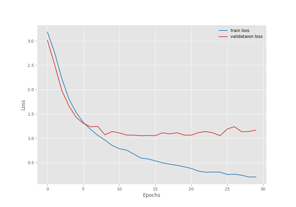
As seen from the above graph, the validation loss starts to increase after 25 epochs.

Testing the Trained Models

The test.py script contains the code to test the model on the held-out test set.

We need to provide the path to the weights file. In all cases, we will use the best weights that have been saved during training.

The following commands show the running of the test script for all three models and their outputs.

Testing EfficientNetB0

python test.py --weights ../outputs/efficientnetb0/best_model.pth

Outputs

[INFO]: Freezing hidden layers...
Testing model
100%|█████████████████████████████████████████████| 236/236 [00:13<00:00, 17.68it/s]
Test accuracy: 64.407%

Testing ResNet18

python test.py --weights ../outputs/resnet18/best_model.pth

Outputs

[INFO]: Freezing hidden layers...
Testing model
100%|█████████████████████████████████████████████| 236/236 [00:10<00:00, 23.36it/s]
Test accuracy: 58.898%

Testing ResNet50

python test.py --weights ../outputs/resnet50/best_model.pth

Outputs

[INFO]: Freezing hidden layers...
Testing model
100%|█████████████████████████████████████████████| 236/236 [00:08<00:00, 26.81it/s]
Test accuracy: 66.525%

The results are quite interesting. If you remember, EfficientNetB0 had the best validation accuracy according to the model that we saved. But on the test set, EfficientNetB0 is performing worse than ResNet50.

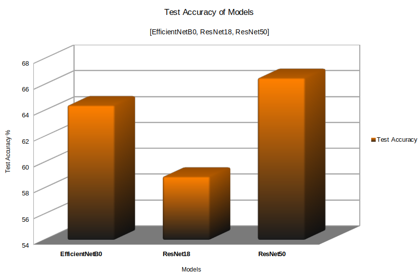
ResNet50 achieves a test accuracy of 66.525% whereas EfficieNetB0 achieves 64.407%. ResNet18 achieves the least test accuracy of 58.898%.

ResNet50 is able to correctly classify a few more images with diverse backgrounds compared to EfficieNetB0.

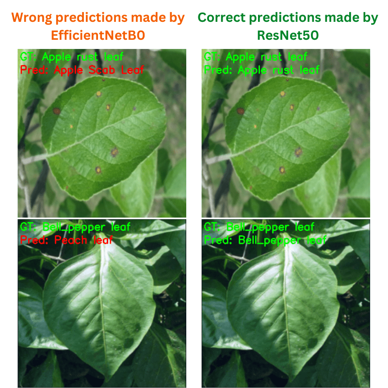
The above figure shows some plant diseases that ResNet50 is able to recognize correctly but EfficientNetB0 cannot. It seems that ResNet50 has learned the background feature better compared to EfficientNetB0.

Inference on Real-World Images of Leaves Affected by Diseases

Let’s use the ResNet50 model to run inference on some real-world images of leaves that have been affected by a specific disease.

The inference.py script contains the code for inference. We just need to provide the path to the weights and the script will run inference on the images present in input/inference_data. The image file names indicate the disease and plant.

python inference.py --weights ../outputs/resnet50/best_model.pth

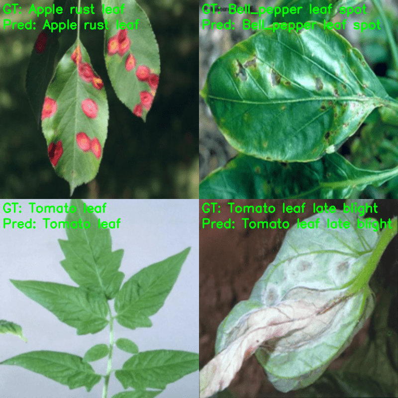
The following figure shows the results. The text in blue color shows the ground truth and the text in red color (annotated using OpenCV in the inference.py script) shows the predictions.

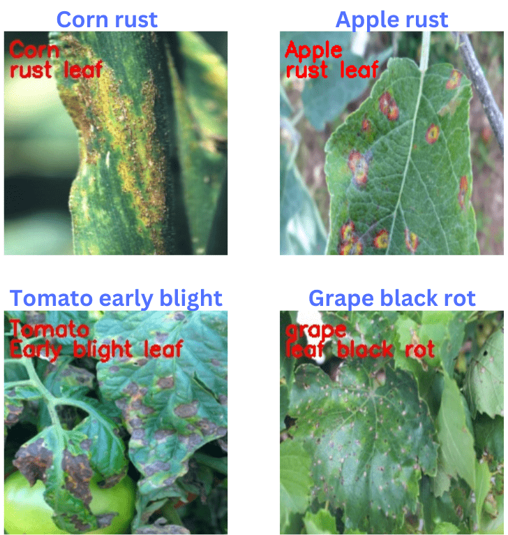
As we can see, ResNet50 is able to recognize all the plants and their diseases correctly. In fact, it is able to recognize the tomato early blight and corn rust correctly which the EfficienNetB0 trained on the PlantVillage dataset was not able to recognize correctly.

This shows how when training images contain enough diversity and real-world samples, we always do not need tens of thousands of images to train a good model. Although the larger the dataset, the better it is, a few thousand quality samples can be much more valuable to train a good model.

Summary and Conclusion

In this blog post, we carried out a small experimental project by training three different image classification models on the PlantDoc dataset. After training and testing the models, we got to know how larger models generally perform better on complex datasets. The experiments also made clear that the test accuracy does not always resemble the real-world performance of a deep learning model. I hope that you learned something new from this post.

If you have any doubts, thoughts, or suggestions, please leave them in the comment section. I will surely address them.

You can contact me using the Contact section. You can also find me on LinkedIn, and Twitter.

Inference Image Credits

• apple_rust.jpg
• tomato_blight.jpg
• corn_rust.jpg
• grape_black_rot.jpg