UAV Small Object Detection using Deep Learning and PyTorch

Small object detection is a real challenge for deep learning models. Most deep learning models, although capable of performing well when detecting large objects, perform relatively worse on small objects. Even more so, when we start to fine-tune an object detection model on a new dataset. In this tutorial, we will carry out UAV Small Object Detection. In short, we will train an object detection model on high-resolution aerial imagery which contains very small objects. This will be a nice challenge considering that we will deal with a very unique dataset.

Capturing drone imagery and performing visual analysis on them is growing nowadays. Image recognition, detection, and segmentation play a big part in these analyses. As such, deep learning models remain at the forefront of such applications. This post will act as a starting point for us to know the capabilities and limitations of such models on small object detection from UAVs.

We are going to cover the following points in this tutorial:

• We will start with a discussion of the dataset. This will help us get familiar with the UAV Small Object Detection dataset.
• Then we will discuss the Python scripts that we need to get the training procedure going. This will also include the deep learning model that we will use.
• Next, we will focus on the training and evaluation of the model.
• Finally, we will analyze the results on the test dataset and discuss how we can improve the performance of the model.

The UAV Small Object Detection Dataset

We will use the UAVOD-10 dataset to train our object detection model on small objects in this tutorial. The original dataset is available on GitHub but we will use a slightly different version of it. It also has an associated paper – A context-scale-aware detector and a new benchmark for remote sensing small weak object detection in unmanned aerial vehicle images by Han et al.

The paper shows a new method, context-scale-aware architecture for small object detection. But we will use a COCO pretrained model from Torchvision here and see how far it takes us.

The original dataset contains 844 images across 10 different classes. The annotations are present in XML format and here are the exact class names from the XML files.

• building
• ship
• vehicle
• prefabricated-house
• well
• cable-tower
• pool
• landslide
• cultivation-mesh-cage
• quarry

The original dataset does not contain a train, validation, and test split. So, I created these splits and uploaded the dataset on Kaggle under open access. Please download the dataset from Kaggle if you wish to run the training script from this tutorial. After splitting, there are 717 training, 84 validation, and 43 test samples respectively.

After downloading the dataset, you should get the following directories.

├── test_annots [43 entries exceeds filelimit, not opening dir]
├── test_images [43 entries exceeds filelimit, not opening dir]
├── train_annots [717 entries exceeds filelimit, not opening dir]
├── train_images [717 entries exceeds filelimit, not opening dir]
├── valid_annots [84 entries exceeds filelimit, not opening dir]
└── valid_images [84 entries exceeds filelimit, not opening dir]

Further in the article, we will see how to structure the entire directory for the project.

Objects In the Dataset

Although there are only 844 images in the dataset, the total number of instances is 18,234. All the images are in high resolution. Starting from 1600 pixels in width, some even go up to 2700 pixels in width.

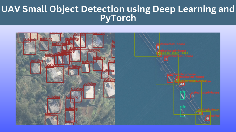
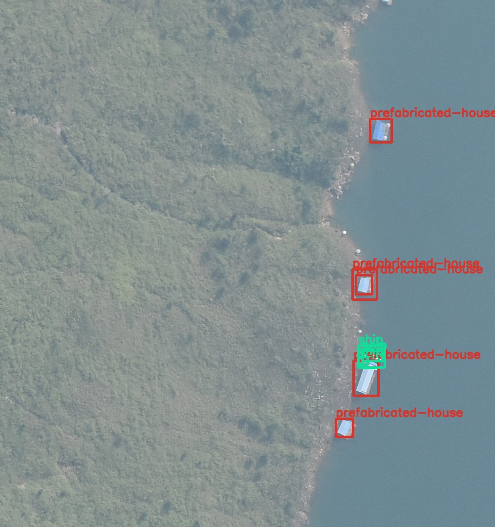
The images were captured from an Unmanned Aerial Vehicle and most of the objects appear quite small. Here are some samples with their annotations.

The above image contains a well among other objects. We can see that the well appears very small and it is one of the smallest instances in the entire dataset.

In the above figure, we can see ships and pre-fabricated houses. Both of them can be present near the water and can sometimes be even confused for the same objects.

Training an object detection model on these UAV images will be challenging. In the end, we will also discuss all the approaches that did not work.

Project Directory Structure

Let’s go over the directory structure for the project.

├── data
│   ├── test_annots
│   ├── test_images
│   ├── train_annots
│   ├── train_images
│   ├── valid_annots
│   └── valid_images
├── inference_outputs
│   └── images
├── notebooks
│   └── visualizations.ipynb
├── outputs
│   ├── best_model.pth
│   ├── last_model.pth
│   ├── map.png
│   └── train_loss.png
├── config.py
├── custom_utils.py
├── datasets.py
├── eval.py
├── inference.py
├── model.py
└── train.py

• The data directory contains the downloaded and extracted dataset. In case, the extracted dataset is in another subdirectory, please arrange it like the above where the split directories are directly inside the data directory.
• The inference_outputs and outputs directories contain the outputs from inference and training respectively.
• We have a notebooks directory with a notebook for visualizing the images with annotations.
• Directly inside the project directory, we have 7 Python scripts. We will discuss the purpose of each of these in the coding section.

Downloading the zip file for this tutorial will give you access to all the code files and the best trained weights. You can run inference using the weights. If you wish to train the model, you will need to download the dataset from Kaggle and arrange it as shown in the above structure.

The code in this tutorial uses PyTorch 2.0.0. But any version starting from PyTorch 1.12.0 should work.

Small Object Detection From UAV Images using PyTorch and Deep Learning

While training the model in this tutorial, we completely rely on our own methodologies and a COCO pretrained model. We do not choose the best object detection model for the detection of small objects from a UAV.

As there are 7 Python scripts, we will not go into the details of all of these. We will go into the most important code sections for sure, but please feel free to explore the code on your own if you wish to understand the pipeline.

Download Code

The Configuration File

We have a config.py file in our code base. It has some predefined configurations which makes the training process a bit simpler. Let’s go through its contents.

import torch

BATCH_SIZE = 4 # Increase / decrease according to GPU memeory.
RESIZE_TO = 1000 # Resize the image for training and transforms.
NUM_EPOCHS = 55 # Number of epochs to train for.
NUM_WORKERS = 4 # Number of parallel workers for data loading.

DEVICE = torch.device('cuda') if torch.cuda.is_available() else torch.device('cpu')

# Training images and XML files directory.
TRAIN_IMG = 'data/train_images'
TRAIN_ANNOT = 'data/train_annots'
# Validation images and XML files directory.
VALID_IMG = 'data/valid_images'
VALID_ANNOT = 'data/valid_annots'

# Classes: 0 index is reserved for background.
CLASSES = [
    '__background__',
    'building',
    'ship',
    'vehicle',
    'prefabricated-house',
    'well',
    'cable-tower',
    'pool',
    'landslide',
    'cultivation-mesh-cage',
    'quarry'
]

NUM_CLASSES = len(CLASSES)

# Whether to visualize images after crearing the data loaders.
VISUALIZE_TRANSFORMED_IMAGES = False

# Location to save model and plots.
OUT_DIR = 'outputs'

First, we define a few constants related to the dataset preparation. These are the batch size, the dimensions to resize the images to, and the number of workers for data loading. We also define the number of epochs to train for, which is 55 in this case.

Next, we define the path to the images and annotations directories for both training and validation.

There is a CLASSES list containing all the class names which will be used in dataset preparation. The first class is reserved for __background__ that we can see in the above code block.

Then, we have a VISUALIZE_TRANSFORMED_IMAGES variable. If it is True, then executing the training script will show a few of the transformed images first before starting the training. We keep it False to have an uninterrupted training process.

Finally, we define the directory name where all the training results will be saved.

Faster RCNN ResNet50 FPN V2 for UAV Small Object Detection

Although we will not make any changes to the model architecture for small object detection, still, we will need a good model. Among all the pretrained Torchvision models, the Faster RCNN ResNet50 FPN V2 has the best metrics on the COCO dataset. We will go ahead and configure that for the small object detection from UAV.

This is the code in the model.py file containing everything that we need to prepare the model.

import torchvision

from torchvision.models.detection.faster_rcnn import FastRCNNPredictor

def create_model(num_classes=91):
    model = torchvision.models.detection.fasterrcnn_resnet50_fpn_v2(
        weights='DEFAULT'
    )
    # Get the number of input features .
    in_features = model.roi_heads.box_predictor.cls_score.in_features
    # Define a new head for the detector with required number of classes.
    model.roi_heads.box_predictor = FastRCNNPredictor(in_features, num_classes)

    return model

if __name__ == '__main__':
    model = create_model(4)
    print(model)
    # Total parameters and trainable parameters.
    total_params = sum(p.numel() for p in model.parameters())
    print(f"{total_params:,} total parameters.")
    total_trainable_params = sum(
        p.numel() for p in model.parameters() if p.requires_grad)
    print(f"{total_trainable_params:,} training parameters.")

All the model preparation code is in the create_model() function. It accepts num_classes as a parameter which is the number of classes in the dataset.

On line 6, we load the model architecture along with the pretrained weights. The 'DEFAULT' argument will load the best available weights.

Next, we get the input features and modify the classification and bounding box regression layers on line 12.

Executing model.py will print the model architecture and the number of parameters.

python model.py

python model.py 
FasterRCNN(
  (transform): GeneralizedRCNNTransform(
      Normalize(mean=[0.485, 0.456, 0.406], std=[0.229, 0.224, 0.225])
      Resize(min_size=(800,), max_size=1333, mode='bilinear')
  )
  (backbone): BackboneWithFPN(
    (body): IntermediateLayerGetter(
      (conv1): Conv2d(3, 64, kernel_size=(7, 7), stride=(2, 2), padding=(3, 3), bias=False)
      (bn1): BatchNorm2d(64, eps=1e-05, momentum=0.1, affine=True, track_running_stats=True)
      (relu): ReLU(inplace=True)
      (maxpool): MaxPool2d(kernel_size=3, stride=2, padding=1, dilation=1, ceil_mode=False)
      (layer1): Sequential(
.
.
.
(box_predictor): FastRCNNPredictor(
      (cls_score): Linear(in_features=1024, out_features=4, bias=True)
      (bbox_pred): Linear(in_features=1024, out_features=16, bias=True)
    )
  )
)
43,266,403 total parameters.
43,266,403 training parameters.

The Dataset Preparation Code and Other Utility Code

We will not into all the details of the dataset preparation code and utility code. They are quite long. But please feel free to go over them before starting the training process.

We will discuss a few caveats about the dataset and how we are handling them here. In the datasets.py file, there are these lines of code.

# Check that max coordinates are at least one pixel
# larger than min coordinates.
if xmax_final == xmin_final:
    xmin_final -= 1
if ymax_final == ymin_final:
    ymin_final -= 1
# Check that all coordinates are within the image.
if xmax_final > self.width:
    xmax_final = self.width
if ymax_final > self.height:
    ymax_final = self.height

So, what does this exactly do and why do we need them?

The UAV small object detection dataset contains a few objects where the xmin (top-left) and xmax (bottom-right) are at the same pixel location. And after resizing and normalization when passing through the albumentations augmentations for bounding boxes, it throws up an error. Instead of discarding such images, we just reduce the size of the xmin by 1 pixel. Mostly, it does not harm and the xmax is now at least one pixel bigger than xmin.

Next, we do another check. Sometimes, the dataset may contain xmax and ymax pixels such that they go out of the boundary of the image. We are almost certain that the visibility of the object ends at the boundary and therefore, make the xmax and ymax equal to the width and height of the image respectively.

Next, coming to the custom_utils.py script. This also contains quite a few important pieces of code. These include code to save the best model weights, the last model weights, class to calculate the average loss, and saving the mAP & loss plots.

Data Augmentations

Another important piece of code is the data augmentation. We stick to two augmentation techniques for the UAV small object detection dataset images. They are:

• Horizontal flipping with a probability of 0.5.
• Rotation with a rotation limit of 30 degrees and probability of 0.3.

From experiments, I found that blur, motion blur, and median blur augmentations do not work very well. Most probably, they make the dataset too challenging for the model to learn.

The Training Script

The train.py file contains all the training code. It combines everything, prepares the datasets, and the data loaders, initializes the optimizer, and defines the learning rate scheduler as well.

We use the SGD optimizer with an initial learning rate of 0.01 with a StepLR learning rate scheduler. The scheduler reduces the learning rate by a factor of 10 after 45 epochs.

You can execute the following command from the terminal in the project directory to start the training.

python train.py

The following are the truncated outputs. We are monitoring the mAP metric to determine the best model.

Number of training samples: 717
Number of validation samples: 84
.
.
.
EPOCH 1 of 55
Training
Loss: 0.9593: 100%|████████████████████| 180/180 [01:01<00:00,  2.91it/s]                                                                                                                     
Validating
100%|████████████████████| 21/21 [00:03<00:00,  5.31it/s]                                                                                                                                     
Epoch #1 train loss: 1.070
Epoch #1 [email protected]:0.95: 0.13552576303482056
Epoch #1 [email protected]: 0.28479906916618347
Took 1.231 minutes for epoch 0

BEST VALIDATION mAP: 0.13552576303482056

SAVING BEST MODEL FOR EPOCH: 1

SAVING PLOTS COMPLETE...
Adjusting learning rate of group 0 to 1.0000e-02.
.
.
.
Epoch #38 train loss: 0.442
Epoch #38 [email protected]:0.95: 0.30711764097213745
Epoch #38 [email protected]: 0.5797217488288879
Took 1.156 minutes for epoch 37

BEST VALIDATION mAP: 0.30711764097213745

SAVING BEST MODEL FOR EPOCH: 38

SAVING PLOTS COMPLETE...
Adjusting learning rate of group 0 to 1.0000e-02.
.
.
.
EPOCH 55 of 55
Training
Loss: 0.2660: 100%|████████████████████| 180/180 [00:58<00:00,  3.08it/s]                                                                                                                     
Validating
100%|████████████████████| 21/21 [00:03<00:00,  5.63it/s]                                                                                                                                     
Epoch #55 train loss: 0.333
Epoch #55 [email protected]:0.95: 0.2849176824092865
Epoch #55 [email protected]: 0.5586428642272949
Took 1.114 minutes for epoch 54
SAVING PLOTS COMPLETE...
Adjusting learning rate of group 0 to 1.0000e-03.

The model reached the best mAP of 30.7% on epoch 38. Let’s take a look at the mAP plot to gain further insights.

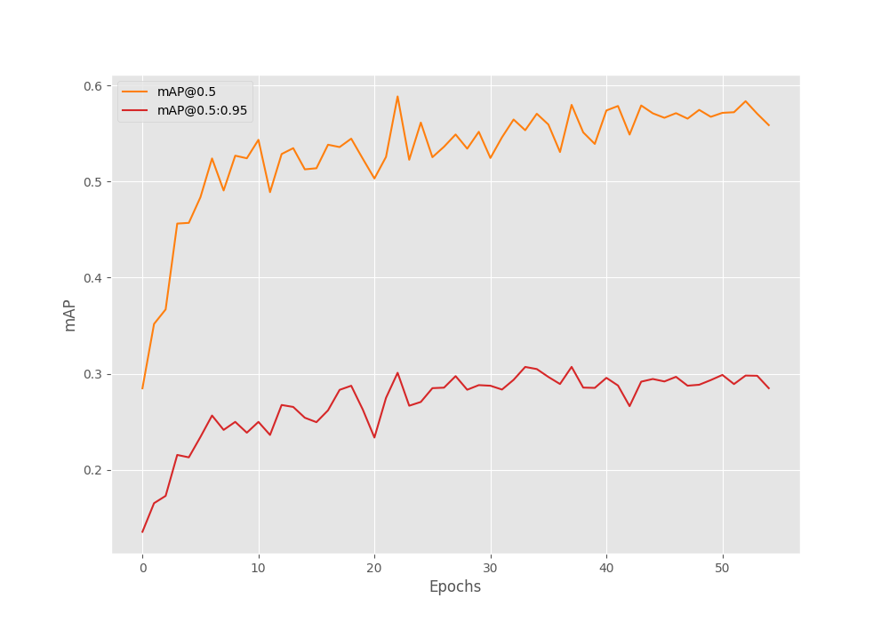
We can see that even after reducing the learning rate, the mAP did not improve, though it was stable. This indicates that we may need to add more augmentation techniques to the dataset to prevent overfitting.

Evaluation on the Test Set

Right now, we have a model that has been trained on the UAV small object detection dataset. We can use the best weights to run an evaluation on the test set.

The eval.py script contains the code for evaluating the model on the test set. We can run the following command to start the evaluation.

python eval.py --weights outputs/best_model.pth --input-images data/test_images/ --input-annots data/test_annots/

We use the following command line arguments in the above command:

• --weights: This accepts the path to the weight file. We are providing the path to the best weights here.
• --input-images: The directory containing the images.
• --input-annots: The directory containing the annotation files.

We get the following results.

mAP_50: 63.755
mAP_50_95: 33.238

The [email protected]:0.95 is 33.23% which is not very bad considering the difficulty of the dataset.

Running Inference on the Test Images and Analyzing the Results Qualitatively

Till now, we have analyzed the results from the UAV small object detection training quantitatively using the mAP metrics. Now, let’s run inference on the test set images and analyze the results manually (qualitatively).

We can run the inference.py script to start the inference process.

python inference.py --weight outputs/best_model.pth --input data/test_images/ --imgsz 1000 --threshold 0.45

We use the following command line arguments:

• --weights: To provide the path to the best trained weight.
• --input: Path to the input directory.
• --imgsz: We pass 1000 for this which will resize the images to 1000×1000 resolution. This is the same resolution as was during training.
• --threshold: This is the score threshold to rule out some less confident results.

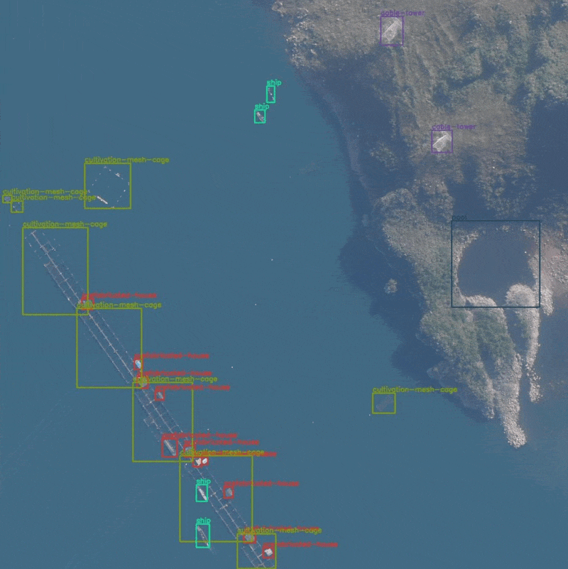
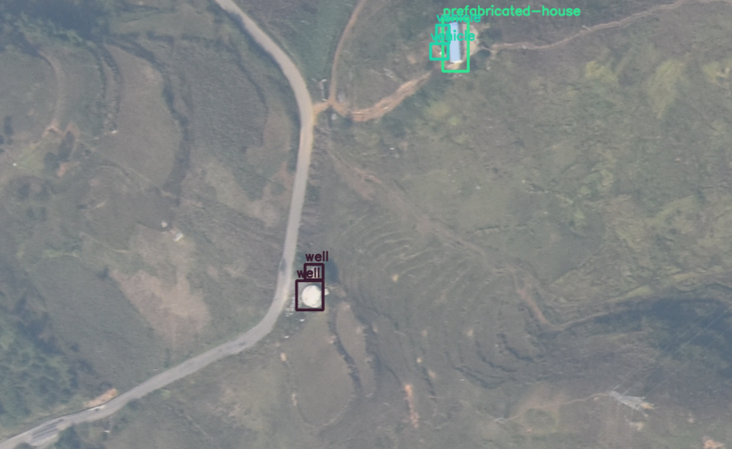
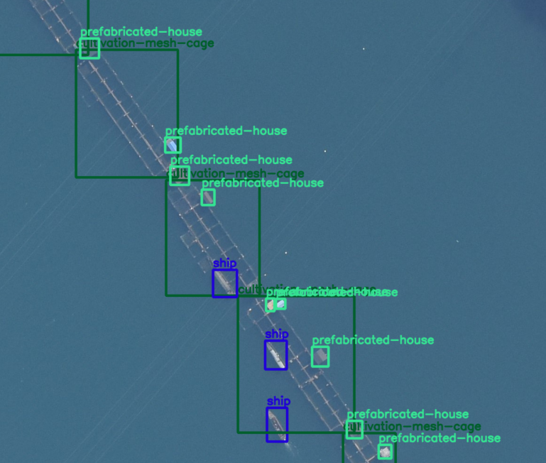
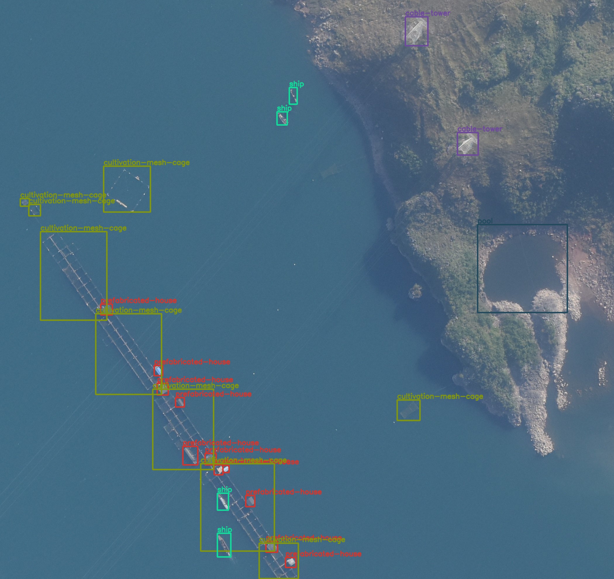
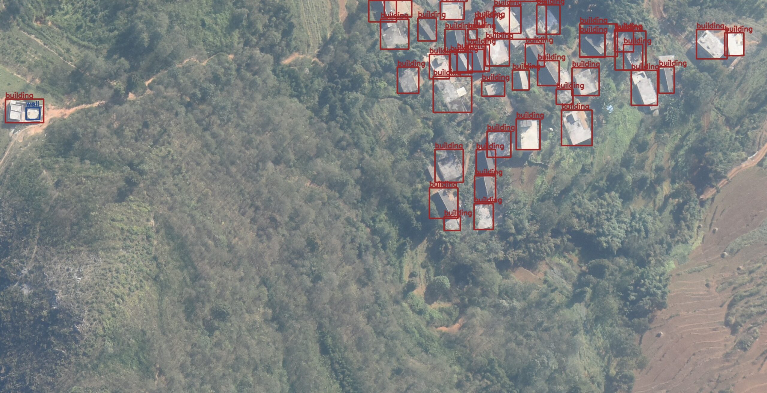
Here are some of the inference results.

You may need to open the images in a new tab and zoom in to get visualize the annotations. Else, the annotations may appear small as these are high-resolution images.

The predictions in the above two images are almost perfect apart from the missing detection of one house in the second image.

Now, let’s take a look at two images where the model clearly made some wrong predictions.

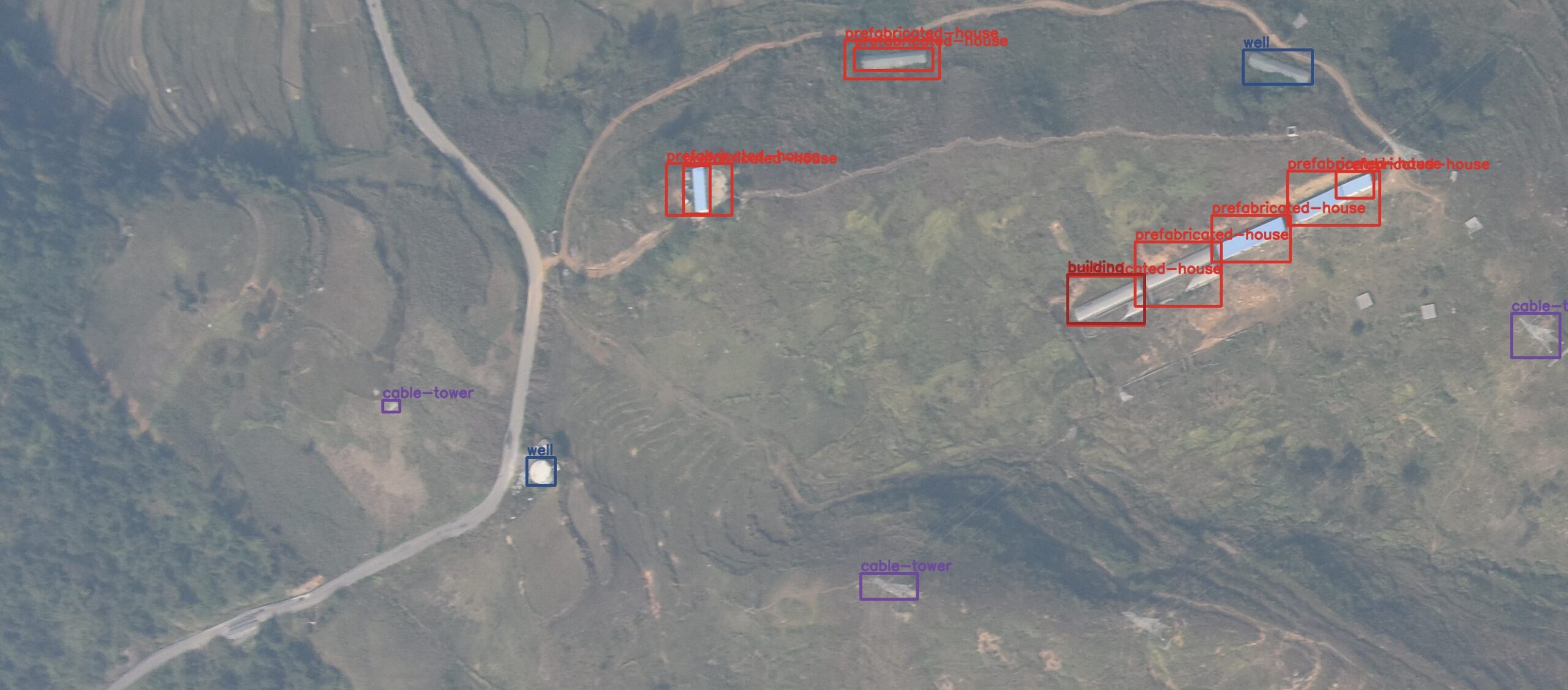
In figure 8, the model is predicting house and ship multiple times for the same instance.

Coming to figure 9, the model is missing the prediction for a well. Moreover, it is wrongly detecting building instance and also missing a detection for a cable-tower.

You can go over the other detections in inference_outputs/images directory and further analyze the results. You can also cross-check the predictions using the visualizations.ipynb notebook.

Configurations Which Did Not Work

Here is a list of configurations and experiments which did not yield good results.

• Lower starting learning rate: Starting from a learning rate of 0.001 or 0.005 did not work very well.
• Blur augmentations: Augmentations such as blur, media blur, and motion blur made the dataset too difficult to learn.
• Lower image resolution: Resizing the images to a lower resolution such as 512×512 made the training process worse. This is mostly because the objects in the images are small.

Summary and Conclusion

In this tutorial, we trained an object detection model from UAV images. The dataset was quite challenging and we had to take some precautionary steps to ensure that the model learned the features well. After inference, we also discussed the results which were good, and also where the model made mistakes. In the end, we also discussed a few points that did not work very well for the training experiments. I hope that the tutorial was worth your time.

If you have any doubts, thoughts, or suggestions, please leave them in the comment section. I will surely address them.

You can contact me using the Contact section. You can also find me on LinkedIn, and Twitter.