
Exporting deep learning models to different formats is essential to model deployment. One of the most common export formats is ONNX (Open Neural Network Exchange). Converting to ONNX optimizes the model to utilize the capabilities of the deployment platform effectively. These can include Intel CPUs, NVIDIA GPUs, and even AMD GPUs with ROCm capability. However, getting started with converting models to ONNX can be challenging, even more so when using the converted model for inference. In this article, we will simplify the process. We will export a custom PyTorch object detection model to ONNX. Not only that, but we will also learn how to use the exported ONNX model for inference with CUDA support.
While doing so, we will follow all the steps in this article. Starting from the training of the model, then exporting the PyTorch Model to ONNX, and finally carrying out inference.
Let’s check out all the points that we will discuss in this article.
- As usual, we will start with a short discussion of the dataset. We will use a simple person detection dataset.
- We will follow that with the setting up of the environment.
- Then, we will discuss the components of the training script in brief. As our primary focus is the export of the PyTorch model to ONNX, we will not go in-depth into the training code explanation.
- Next, we will go through the script to export the PyTorch detection model to ONNX. In this part, we will also discuss some of the caveats that we need to take care of.
- After the ONNX conversion, we will again carry out inference using the exported model using the ONNX CUDA Execution Provider.
The Person Detection Dataset
In this article, we will use a simple person detection dataset to fine-tune a COCO pretrained RetinaNet model from Torchvision.
The only reason to choose this dataset is that it is simple to train on and we can expect very good results. You can find the person detection dataset on Kaggle. Please go ahead and download the dataset for now.
It contains 944 training, 160 validation, and 235 test samples. All the annotations are in XML format. Here are some of the ground truth images with their annotations.
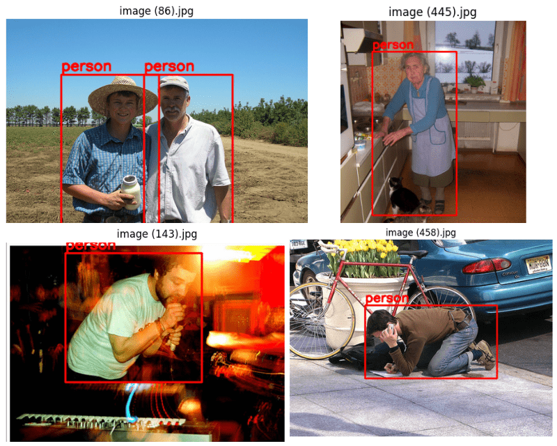
There is only one class in the dataset, that is, person.
After downloading the extracting the dataset, you should get the following directory structure.
.
├── Test
│   └── Test
│       └── JPEGImages
├── Train
│   └── Train
│       └── JPEGImages
└── Val
    └── Val
        └── JPEGImages
Both, the images and the XML files are present inside the JPEGImages directory for all three splits. In the next section, we will organize the entire project’s directory structure.
PyTorch Model ONNX Export Project Directory Structure
We have the following directory structure for the entire project.
├── data
│   ├── inference_data
│   ├── Test
│   ├── Train
│   └── Val
├── inference_outputs
│   └── videos
├── notebooks
│   └── visualizations.ipynb
├── outputs
│   ├── best_model.pth
│   ├── last_model.pth
│   ├── map.png
│   └── train_loss.png
├── weights
│   └── model.onnx
├── config.py
├── custom_utils.py
├── datasets.py
├── env_setup_commands.txt
├── eval.py
├── export.py
├── inference.py
├── inference_video.py
├── model.py
├── onnx_inference_video.py
├── requirements.txt
└── train.py
- The data directory contains the downloaded dataset that we saw in the previous section. Along with that, it also contains an
inference_datasubdirectory with videos that we will use for inference. - The inference and training outputs will go into the
inference_outputsandoutputsdirectories respectively. - We also have a
notebooksdirectory containing a Jupyter Notebook for data visualization. - The
weightsfolder will hold the exported ONNX model. - Directly inside the parent project directory, we have several Python files. As we move along the article, we will go into the explanation of the necessary files.
- We also have an
env_setup_commands.txtandrequirements.txtto help us set up our local environment. We will discuss this in detail in the next section.
All the code files, weights, and the exported ONNX model will be available through the downloadable zip file. If you wish to run the training as well, please download the dataset as well and arrange it in a structure similar to the above.
Setting Up the Local Environment
Setting up the local environment is essential to both, the training and running the exported ONNX model on the GPU. We will need the right versions of PyTorch, CUDA, and ONNX runtime.
The env_setup_commands.txt contains all the commands that we need to set up an environment locally using conda. Furthermore, the requirement.txt file contains all the specific package versions.
Apart from the creation of a new environment, we will go through the rest of the commands here to set up the local environment to export PyTorch models into ONNX format. Please follow through with the commands after creating a new environment.
Download Code
First, we need to install PyTorch with CUDA support. We need PyTorch 1.12.1 and CUDA 11.3 in this case.
pip install torch==1.12.1+cu113 torchvision==0.13.1+cu113 torchaudio==0.12.1 --extra-index-url https://download.pytorch.org/whl/cu113
Second, we need to install albumentations for augmentations without OpenCV support. We need albumentations for training the RetinaNet model.
pip install -U albumentations --no-binary qudida,albumentations
Finally, we need to install the rest of the requirements from the requirements.txt file.
pip install -r requirements.txt
That’s all we need to set up the local environment for ONNX export and execution.
Export PyTorch Model to ONNX
From here on, we will go through the practical steps of converting a custom trained PyTorch RetinaNet model to ONNX format. The steps will be as follows:
- First, we will train the RetinaNet model on the person detection dataset.
- Second, we will export the best trained weights to ONNX format.
- Third, we will run inference using the exported ONNX model with CUDA support.
Note: Achieving the best mAP metric is not the goal here. Rather, we will focus on the export and execution of the ONNX model.
Training the RetinaNet Model
Although we will not go through the details of the training code, still we will have an overview of all the files involved in training.
datasets.py
The datasets.py file creates the datasets and data loaders for the training script. While creating the datasets, we are also applying some minor augmentations to prevent overfitting. These include:
- Horizontal flipping
- Rotation
You can also execute the datasets.py file to visualize a few images decoded from the data loaders. This will show the exact images that go into the model while training.
custom_utils.py
This file contains all the helper functions and utility classes. These include classes to save the best model and track the training error. Along with that it also contains functions to plot the mAP and loss graphs. The functions to define the augmentations are also in this file.
config.py
This file defines all the configurations needed for training. These include:
- The batch size for data loaders, we are using a batch size of 8.
- The resize factor. All the images will be resized to 640×640 resolution.
- Number of workers for the data loaders. It is 4 in our case.
- The computation device. Whether to use the CPU or GPU.
- The class names and paths to the images and annotations folders.
Other scripts import the necessary constants from the configuration file as and when needed.
train.py
This is the executable script to start the training. We use the SGD optimizer with a starting learning rate of 0.01 and momentum of 0.9. A Step Learning Rate scheduler will reduce the learning rate to 0.001 after 10 epochs. We will train for a total of 20 epochs as defined in the config.py file.
Note: The following training and inference experiments were conducted on a machine with 10 GB RTX 3080 GPU, 10th generation i7 CPU, and 32 GB RAM.
Let’s start the training. We can execute the following command in the terminal to start the training.
python train.py
Here is the truncated output from the terminal.
Number of training samples: 944
Number of validation samples: 160

RetinaNet(
  (backbone): BackboneWithFPN(
    (body): IntermediateLayerGetter(
      (conv1): Conv2d(3, 64, kernel_size=(7, 7), stride=(2, 2), padding=(3, 3), bias=False)
      (bn1): BatchNorm2d(64, eps=1e-05, momentum=0.1, affine=True, track_running_stats=True)
      (relu): ReLU(inplace=True)
      (maxpool): MaxPool2d(kernel_size=3, stride=2, padding=1, dilation=1, ceil_mode=False)
.
.
.
36,352,630 total parameters.
36,127,286 training parameters.
Adjusting learning rate of group 0 to 1.0000e-02.

EPOCH 1 of 20
Training
Loss: 0.3569: 100%|████████████████████| 118/118 [00:54<00:00,  2.18it/s]
Validating
100%|████████████████████| 20/20 [00:04<00:00,  4.16it/s]
Epoch #1 train loss: 0.901
Epoch #1 [email protected]:0.95: 0.30067628622055054
Epoch #1 [email protected]: 0.5657806396484375
Took 1.183 minutes for epoch 0

BEST VALIDATION mAP: 0.30067628622055054

SAVING BEST MODEL FOR EPOCH: 1

SAVING PLOTS COMPLETE...
Adjusting learning rate of group 0 to 1.0000e-02..
.
.
.
EPOCH 20 of 20
Training
Loss: 0.2828: 100%|████████████████████| 118/118 [00:48<00:00,  2.42it/s]
Validating
100%|████████████████████| 20/20 [00:04<00:00,  4.77it/s]
Epoch #20 train loss: 0.180
Epoch #20 [email protected]:0.95: 0.6373328566551208
Epoch #20 [email protected]: 0.9279314279556274
Took 0.939 minutes for epoch 19

BEST VALIDATION mAP: 0.6373328566551208

SAVING BEST MODEL FOR EPOCH: 20

SAVING PLOTS COMPLETE...
Adjusting learning rate of group 0 to 1.0000e-04.
The mAP metric kept improving till the end of training and we have the best mAP of 63.73% on the validation set after 20 epochs.
The following are the training loss and validation mAP graphs.
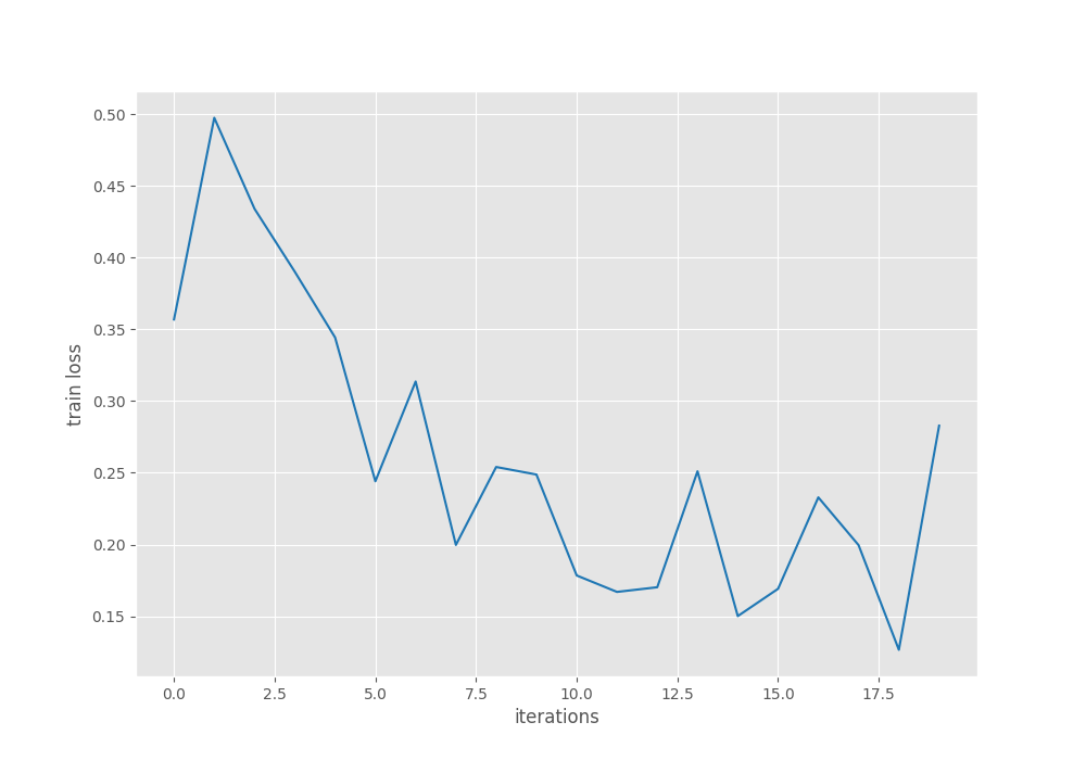
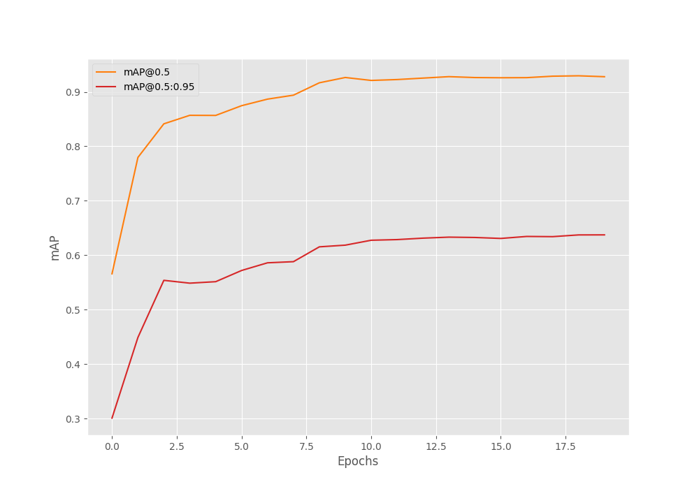
Although the loss graph seems to be fluctuating a bit, the mAP graph seems to be improving quite steadily. Perhaps the model can be trained for a few more epochs.
We can also execute the eval.py script with the following command to run evaluation on the test data.
python eval.py
100%|███████████████| 30/30 [00:09<00:00,  3.10it/s]
mAP_50: 89.423
mAP_50_95: 55.540
We got an mAP of 55.540% which is not very bad.
Further, we can also use the inference.py and inference_video.py scripts to run inference using the PyTorch model. But here, we will move on to the export of the RetinaNet model to ONNX format.
Exporting the RetinaNet Model to ONNX Format
The export.py file contains all the code for exporting the model to ONNX format. Let’s take a look at the code first, then we will go into the explanation.
import torch
import argparse
import os

from model import create_model
from config import (
    DEVICE, NUM_CLASSES
)

def parse_opt():
    parser = argparse.ArgumentParser()
    parser.add_argument(
        '-w', '--weights',
        default=None,
        help='path to trained checkpoint weights if providing custom YAML file'
    )
    parser.add_argument(
        '-d', '--device',
        default=torch.device('cuda:0' if torch.cuda.is_available() else 'cpu'),
        help='computation/training device, default is GPU if GPU present'
    )
    parser.add_argument(
        '--out',
        help='output model name, e.g. model.onnx',
        required=True,
        type=str
    )
    parser.add_argument(
        '--width',
        default=640,
        type=int,
        help='onnx model input width'
    )
    parser.add_argument(
        '--height',
        default=640,
        type=int,
        help='onnx model input height'
    )
    args = parser.parse_args()
    return args

def main(args):
    OUT_DIR = 'weights'
    if not os.path.exists(OUT_DIR):
        os.makedirs(OUT_DIR)
    # Load weights if path provided.
    # Load the best model and trained weights.
    model = create_model(num_classes=NUM_CLASSES)
    checkpoint = torch.load(args.weights, map_location=DEVICE)
    model.load_state_dict(checkpoint['model_state_dict'])
    model.eval()

    # Input to the model
    x = torch.randn(1, 3, args.width, args.height, requires_grad=True)

    # Export the model
    torch.onnx.export(
        model,
        x,
        os.path.join(OUT_DIR, args.out),
        export_params=True,
        opset_version=13,
        do_constant_folding=True,
        input_names=['input'],
        output_names = ['output'],
        dynamic_axes={
            'input' : {0 : 'batch_size'},
            'output' : {0 : 'batch_size'}
        }
    )
    print(f"Model saved to {os.path.join(OUT_DIR, args.out)}")

if __name__ == '__main__':
    args = parse_opt()
    main(args)
Frankly, the code is not very long for exporting the model to ONNX format.
We import all the necessary modules and libraries from lines 1 to 8.
Then we define all the command line arguments. Some of the important ones are:
--weights: The path to the trained weights file that we want to convert to ONNX.--out: The name of the ONNX model file. If we passmodel.onnx, then the final model will be saved inweights/model.onnxpath.--widthand--height: It is important to export the ONNX model for a specific width and height. While running inference using the ONNX model, we have to resize the images/frames to the same size as the model was exported with. Here both, width and height are 640.
In the main() function, first we load the model weights from lines 49 to 52. We define an input to the model on line 55. This will be used as an input while exporting.
We use the export() function from the torch.onnx module to export the model. The first three arguments are the model, an input tensor, and the output path where the ONNX model will be saved.
To export the model to ONNX format, we need to execute the following command.
python export.py --weights outputs/best_model.pth --out model.onnx
In the above command:
--weightsis the path to the trained PyTorch weights.--outis the name of the ONNX model that will be saved in theweightsdirectory.
Note: You may see a few warnings during the export process, but there is nothing to worry about.
Inference Using the Exported Model
We have the exported ONNX model with us now. There is an onnx_inference_video.py file that contains the code for carrying out inference on videos using the ONNX model.
There are two important parts to the script. The first one is the definition of the ONNX runtime session. Here we load the model.
##### PART OF onnx_inference_video.py #####
# Load model.
ort_session = onnxruntime.InferenceSession(
    args.weights, providers=['CUDAExecutionProvider', 'CPUExecutionProvider']
)
We need to import onnxruntime module and instantiate the session using InferenceSession. The first argument that we pass is the path to the ONNX model weight file. The next argument is providers. We are passing ['CUDAExecutionProvider', 'CPUExecutionProvider']. This means that first, the runtime session will look for a CUDA device. If found, the session will be executed on the CUDA device. If not, the session will be executed on the CPU device. There are providers for other hardware such as AMD as well.
We also have a simple function to convert PyTorch tensors to NumPy before feeding them to the model.
##### PART OF onnx_inference_video.py #####
def to_numpy(tensor):
    return tensor.detach().cpu().numpy() if tensor.requires_grad else tensor.cpu().numpy()
The next important part is the forward pass through the model. It happens within the while loop as we are looping over the video frames.
##### PART OF onnx_inference_video.py #####
preds = ort_session.run(
                output_names=None,
                input_feed={ort_session.get_inputs()[0].name: to_numpy(image_input)}
            )
We need to call the run() method of the ort_session that we initialized above. The first argument, output_names is None. So, the outputs will be lists. The second argument is the input_feed. This requires the PyTorch tensor input converted to NumPy.
If you wish to get a detailed look at the code, please go through the onnx_inference_video.py script once.
We can execute the following command to run inference on videos.
python onnx_inference_video.py --imgsz 640 --input data/inference_data/video_1.mp4 --threshold 0.5
We are passing --imgsz as 640 which will resize all frames to 640×640 before feeding them to the model. This is a necessity as we exported the model with the same shape. Other than that, we are passing the path to the input file and also a score threshold of 0.5.
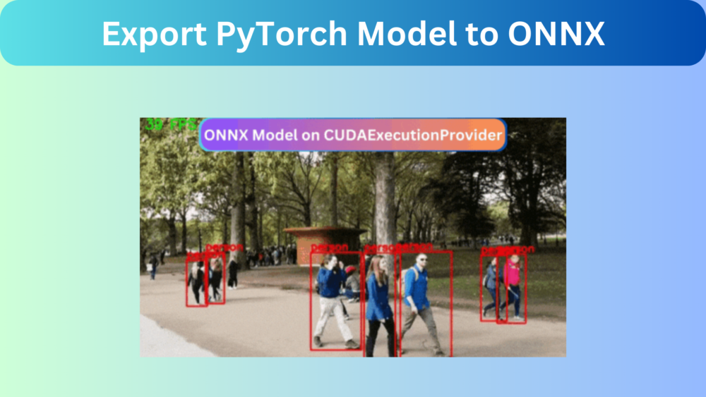
ONNX Inference Video Results
Here are a few results after running the script.
The FPS varies between 39 and 44. If running on a CPU, it would have been somewhere around 1 to 5 FPS. Although results are not the focus of this article, still the results look good. Training for longer will give even better results.
Try running inference on a few of your own videos and let us know about the results in the comment section.
Conclusion
In this article, we learned how to export a PyTorch RetinaNet model to ONNX format. Not only that, after exporting we also ran inference on videos while discussing the important details. If you wish, now you can train and export your own models and even run on different hardware. I hope that this article was useful to you.
If you have any doubts, thoughts, or suggestions, please leave them in the comment section. I will surely address them.
You can contact me using the Contact section. You can also find me on LinkedIn, and X.

How can i download code
Hello Gaurav. Can you please tell me what issue you are facing?