Train PyTorch RetinaNet on Custom Dataset

The Torchvision library of PyTorch has a lot of pretrained models. One of them is the RetinaNet model. It is a single stage object detection model trained on the COCO dataset. Obviously, we can use this pretrained model for inference. But we can easily configure the PyTorch RetinaNet model to fine tune it on the custom datasets. In this article, we will learn how to train the PyTorch RetinaNet object detection model on custom datasets.

Training object detection models from scratch can be difficult. And a lot of times, we may not want to use external libraries to solve an object detection problem. If you are a regular PyTorch user then you can directly use the pretrained object detection models from Torchvision and train them on your own dataset.

In fact, in the last post, we covered how to fine tune the SSD300 VGG16 using Torchvision on a custom dataset.

Before moving further into the technical parts of the article, let’s take a look a the points that we will cover here.

• We will start with a discussion of the dataset first.
• Then we will cover the model preparation part. To train the PyTorch RetinaNet model on a custom dataset, we need to repurpose its head. We will cover that in this section.
• Next, we will have an overview of the other necessary coding components.
• Then we will train the PyTorch RetinaNet model on our custom dataset.
• After training, we will analyze the results and carry out inference on unseen data.

Note: A lot of code will be similar to the previous SSD300 VGG16 fine tuning post. Most of the changes will be in the RetinaNet model preparation part.

The BCCD Dataset to Train the PyTorch RetinaNet Model

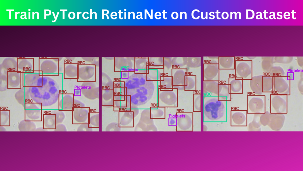
We will use the BCCD dataset to train the PyTorch RetinaNet model. The dataset contains microscopic images of blood cells with 3 classes. The classes are RBC (Red Blood Cells), WBC (White Blood Cells), and Platelets.

We will use the raw Pascal XML version of the dataset which does not contain any augmented images. We will apply our augmentations later while preparing the dataset.

It contains 364 images split into 3 sets, train, validation, and test set. The training set contains 255 images, and the validation set contains 73 images. After training, we will run an evaluation on the test set to get the final mAP (mean average precision). The test set contains 36 images.

The dataset may seem small but it contains enough annotations to train a good RetinaNet model using PyTorch. As such, there are a total of 4888 annotations in the BCCD dataset.

Please ensure to download the dataset before moving further if you intend on training the model on your own.

The PyTorch RetinaNet Training Directory Structure

The following block contains the directory structure of the project.

.
├── data
│   └── BCCD.v3-raw.voc
│       ├── test  [72 entries exceeds filelimit, not opening dir]
│       ├── train  [510 entries exceeds filelimit, not opening dir]
│       ├── valid  [146 entries exceeds filelimit, not opening dir]
│       ├── README.dataset.txt
│       └── README.roboflow.txt
├── inference_outputs
├── outputs
│   ├── best_model.pth
│   ├── last_model.pth
│   ├── map.png
│   └── train_loss.png
├── config.py
├── custom_utils.py
├── datasets.py
├── eval.py
├── inference.py
├── model.py
└── train.py

• The BCCD dataset that we downloaded above resides inside the data directory after extracting it.
• After training, the trained model and the plots will remain in the outputs directory. The inference_outputs directory will contain the results after we run inference on the final test set using the trained model.
• In the project directory, we have 7 Python files. We will focus the most on config.py and model.py in this article. For the others, we will cover the details as per the requirement as the code can be quite long.

You will get access to the best trained weights and the scripts when you download the zip file that comes with this article. In case, you plan on training the model on your own, you will need to download the dataset. Else, you can use the trained model to run evaluation and inference.

Train PyTorch RetinaNet Model on the BCCD Dataset

We will make the codebase as much reusable as possible. Although we use the BCCD dataset to train the PyTorch RetinaNet model in this article, your can train on any dataset of your choice after making slight changes. We will discover more about this as we progress with the coding discussion of the project.

Download Code

The Configuration File

The configuration of the project is one of the most important parts while fine-tuning the RetinaNet model from Torchvision here. This file will contain a lof of predefined settings but we can easily modify them.

All the configurations will go into the config.py file. Here are its contents.

import torch

BATCH_SIZE = 4 # Increase / decrease according to GPU memeory.
RESIZE_TO = 640 # Resize the image for training and transforms.
NUM_EPOCHS = 10 # Number of epochs to train for.
NUM_WORKERS = 4 # Number of parallel workers for data loading.

DEVICE = torch.device('cuda') if torch.cuda.is_available() else torch.device('cpu')

# Training images and XML files directory.
TRAIN_DIR = 'data/BCCD.v3-raw.voc/train'
# Validation images and XML files directory.
VALID_DIR = 'data/BCCD.v3-raw.voc/valid'

# Classes: 0 index is reserved for background.
CLASSES = [
    '__background__', 'RBC', 'WBC', 'Platelets'
]

NUM_CLASSES = len(CLASSES)

# Whether to visualize images after crearing the data loaders.
VISUALIZE_TRANSFORMED_IMAGES = False

# Location to save model and plots.
OUT_DIR = 'outputs'

Let’s go over all the constants that we define in the above configuration file.

• BATCH_SIZE: This defines the batch size for the data loaders. You can increase or decrease it as per the GPU memory available.
• RESIZE_TO: This is the image resize resolution. As per our setting, the dataset preparation code will resize all the images to 640×640 resolution.
• NUM_EPOCHS: The number of epochs to train for. We will train the model for 40 epochs.
• NUM_WORKERS: The number of parallel workers for data loading.
• TRAIN_DIR: This is the directory path containing the training images and annotation files.
• VALID_DIR: This is the directory path containing the validation images and annotations files.
• CLASSES: We are defining the classes present in the dataset in this list. These names should match the names in the XML files. As all the Torchvision pretrained models have a background class, we also add a __background__ class as the first class to the list. According to this, the total number of classes while training Torchvision models should be total number of object classes + the background class.
• NUM_CLASSES: This infers the total number of classes from the CLASSES list.
• VISUALIZE_TRANSFORMED_IMAGES: If this is True, then one sample from the data loader will be shown on the screen before the training starts. This helps us verify that we are feeding the images correctly to the model. For now, we are keeping it False.
• OUT_DIR: This is the name of the output directory where all the training results will be saved.

While training, you can play around with a few parameters, such as RESIZE_TO.

The PyTorch RetinaNet Model

We will use the pretrained RetinaNet model from Torchvision and fine tune it on the BCCD dataset. We will use the new version of the RetinaNet model, that is, retinanet_resnet50_fpn_v2. The following code block contains the entire model preparation code.

import torchvision
import torch

from functools import partial
from torchvision.models.detection import RetinaNet_ResNet50_FPN_V2_Weights
from torchvision.models.detection.retinanet import RetinaNetClassificationHead

def create_model(num_classes=91):
    model = torchvision.models.detection.retinanet_resnet50_fpn_v2(
        weights=RetinaNet_ResNet50_FPN_V2_Weights.COCO_V1
    )
    num_anchors = model.head.classification_head.num_anchors

    model.head.classification_head = RetinaNetClassificationHead(
        in_channels=256,
        num_anchors=num_anchors,
        num_classes=num_classes,
        norm_layer=partial(torch.nn.GroupNorm, 32)
    )
    return model

We do not need to make a lot of changes, but some quite important ones. In the above code block, we define the create_model function which accepts the num_classes as the parameter.

First, we load the pretrained RetinaNet model with the ResNet50 backbone. On line 12, we get the number of anchors. For RetinaNet ResNet50 FPN V2 model, it is 9. This means that there are 9 anchors associated with the layers in the head of the model.

We modify the classification head on line 14. The in_channels=256 defines that each convolutional layer of the classification head will have 256 input channels. This is consistent with the original RetinaNet architecture. Then we provide the number of anchors and the number of classes. The number of classes needs to match the total number of classes in our dataset including the background class.

One important factor is the norm_layer argument. Again, to keep the architecture consistent with the original RetinaNet one, we use the GroupNorm layer with 32 number of groups.

We are skipping the technical details of the individual layers in the above explanation. We discuss the overall architectural change that we need to make to the RetinaNet model to prepare it for a custom dataset.

To make sure that all our changes have taken place effectively, here are the RetinaNet head structures.

  (head): RetinaNetHead(
    (classification_head): RetinaNetClassificationHead(
      (conv): Sequential(
        (0): Conv2dNormActivation(
          (0): Conv2d(256, 256, kernel_size=(3, 3), stride=(1, 1), padding=(1, 1), bias=False)
          (1): GroupNorm(32, 256, eps=1e-05, affine=True)
          (2): ReLU(inplace=True)
        )
        (1): Conv2dNormActivation(
          (0): Conv2d(256, 256, kernel_size=(3, 3), stride=(1, 1), padding=(1, 1), bias=False)
          (1): GroupNorm(32, 256, eps=1e-05, affine=True)
          (2): ReLU(inplace=True)
        )
        (2): Conv2dNormActivation(
          (0): Conv2d(256, 256, kernel_size=(3, 3), stride=(1, 1), padding=(1, 1), bias=False)
          (1): GroupNorm(32, 256, eps=1e-05, affine=True)
          (2): ReLU(inplace=True)
        )
        (3): Conv2dNormActivation(
          (0): Conv2d(256, 256, kernel_size=(3, 3), stride=(1, 1), padding=(1, 1), bias=False)
          (1): GroupNorm(32, 256, eps=1e-05, affine=True)
          (2): ReLU(inplace=True)
        )
      )
      (cls_logits): Conv2d(256, 36, kernel_size=(3, 3), stride=(1, 1), padding=(1, 1))
    )
    (regression_head): RetinaNetRegressionHead(
      (conv): Sequential(
        (0): Conv2dNormActivation(
          (0): Conv2d(256, 256, kernel_size=(3, 3), stride=(1, 1), padding=(1, 1), bias=False)
          (1): GroupNorm(32, 256, eps=1e-05, affine=True)
          (2): ReLU(inplace=True)
        )
        (1): Conv2dNormActivation(
          (0): Conv2d(256, 256, kernel_size=(3, 3), stride=(1, 1), padding=(1, 1), bias=False)
          (1): GroupNorm(32, 256, eps=1e-05, affine=True)
          (2): ReLU(inplace=True)
        )
        (2): Conv2dNormActivation(
          (0): Conv2d(256, 256, kernel_size=(3, 3), stride=(1, 1), padding=(1, 1), bias=False)
          (1): GroupNorm(32, 256, eps=1e-05, affine=True)
          (2): ReLU(inplace=True)
        )
        (3): Conv2dNormActivation(
          (0): Conv2d(256, 256, kernel_size=(3, 3), stride=(1, 1), padding=(1, 1), bias=False)
          (1): GroupNorm(32, 256, eps=1e-05, affine=True)
          (2): ReLU(inplace=True)
        )
      )
      (bbox_reg): Conv2d(256, 36, kernel_size=(3, 3), stride=(1, 1), padding=(1, 1))
    )
  )

We can see that the cls_logits layer in the classification_head has 36 output channels. This is is the result of num_anchors * num_classes. As we have 4 classes including the background, this results in 36 output channels. The regression_head does not change irrespective of the number of classes.

The Dataset Preparation

The dataset preparation part is one of the most important aspects of object detection.

For us, all the dataset preparation code remains in the datasets.py file. In our case, all the annotations are in the XML file format.

The dataset preparation code that we will use, checks some of the important boxes. There are:

• After loading the bounding boxes, it makes sure that all the lower bounds of the coordinates are smaller than the upper bounds of the coordinates. We check this because in some cases, the min and max coordinates may be the same which will result in errors later on in the pipeline.
• The dataset preparation code also ensures that none of the upper-bound coordinates (xmax and ymax) go out of either the width or height of the image. If so, it clips them to the width and height of the image.
• One of the important factors is that we do not discard any image without bounding boxes in the annotation file. We use the images without boxes as background images.

Augmentations

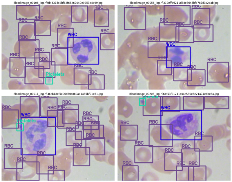
We use a variety of augmentation techniques to avoid overfitting. These include various types of blurring augmentations, flipping, and rotating. As these are images of blood cells, we can safely use the flip and rotate augmentations. However, we need to be careful to not use any color augmentations here as that can compromise how each cell looks. Thus, it may hinder the learning of the RetinaNet model.

Executing datasets.py shows some augmented images and how each image looks before going into the network. Here are some examples.

python datasets.py

With this, we finish the discussion of dataset preparation also.

Helper Functions and Utility Scripts

We also have a custom_utils.py file that contains a few helper functions and classes. These include class to track the training loss, to save the best model, function definitions for the training and validation transforms. Along with these, it also contains the functions to save the mAP and loss plots.

If you are interested, you may have a look at the script before moving further into the training script.

The Training Script

The train.py is the executable script that we run to start the training. In short, it contains the training and validation functions, creates the data loaders, and kicks off the training.

In the train() function we track the training loss, while in the validate() function we use mAP as the evaluation metric for object detection.

We use the Torchmetrics library for calculating the mAP (Mean Average Precision).

To start the training, you can execute the following command in the terminal in the project directory.

python train.py

Here is the truncated output from the terminal.

Number of training samples: 255
Number of validation samples: 73

RetinaNet(
  (backbone): BackboneWithFPN(
    (body): IntermediateLayerGetter(
      (conv1): Conv2d(3, 64, kernel_size=(7, 7), stride=(2, 2), padding=(3, 3), bias=False)
      (bn1): BatchNorm2d(64, eps=1e-05, momentum=0.1, affine=True, track_running_stats=True)
      (relu): ReLU(inplace=True)
      (maxpool): MaxPool2d(kernel_size=3, stride=2, padding=1, dilation=1, ceil_mode=False)
      (layer1): Sequential(
.
.
.
  (transform): GeneralizedRCNNTransform(
      Normalize(mean=[0.485, 0.456, 0.406], std=[0.229, 0.224, 0.225])
      Resize(min_size=(800,), max_size=1333, mode='bilinear')
  )
)
36,394,120 total parameters.
36,168,776 training parameters.
Adjusting learning rate of group 0 to 1.0000e-03.

EPOCH 1 of 40
Training
Loss: 0.8375: 100%|███████████████████████████████████████████████████████████████████████████████████████████████████████████████████████████████████████████| 63/63 [01:10<00:00,  1.11s/it]
Validating
100%|█████████████████████████████████████████████████████████████████████████████████████████████████████████████████████████████████████████████████████████| 18/18 [00:08<00:00,  2.24it/s]
Epoch #1 train loss: 1.017
Epoch #1 mAP: 0.0664602518081665
Took 1.521 minutes for epoch 0

BEST VALIDATION mAP: 0.0664602518081665

SAVING BEST MODEL FOR EPOCH: 1

SAVING PLOTS COMPLETE...

.
.
.
EPOCH 36 of 40
Training
Loss: 0.7795: 100%|███████████████████████████████████████████████████████████████████████████████████████████████████████████████████████████████████████████| 63/63 [02:26<00:00,  2.33s/it]
Validating
100%|█████████████████████████████████████████████████████████████████████████████████████████████████████████████████████████████████████████████████████████| 18/18 [00:17<00:00,  1.05it/s]
Epoch #36 train loss: 0.405
Epoch #36 mAP: 0.580458402633667
Took 2.969 minutes for epoch 35

BEST VALIDATION mAP: 0.580458402633667

SAVING BEST MODEL FOR EPOCH: 36

SAVING PLOTS COMPLETE...
.
.
.
EPOCH 40 of 40
Training
Loss: 0.3943: 100%|███████████████████████████████████████████████████████████████████████████████████████████████████████████████████████████████████████████| 63/63 [02:06<00:00,  2.02s/it]
Validating
100%|█████████████████████████████████████████████████████████████████████████████████████████████████████████████████████████████████████████████████████████| 18/18 [00:17<00:00,  1.01it/s]
Epoch #40 train loss: 0.389
Epoch #40 mAP: 0.572858989238739
Took 2.608 minutes for epoch 39
SAVING PLOTS COMPLETE...

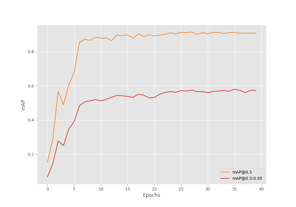
The model reaches the best mAP of 58% on epoch 36.

The mAP here is at IoU 0.50:0.95. So, it seems that the model is doing well. To get even better insights, let’s take a look at the loss and mAP graphs.

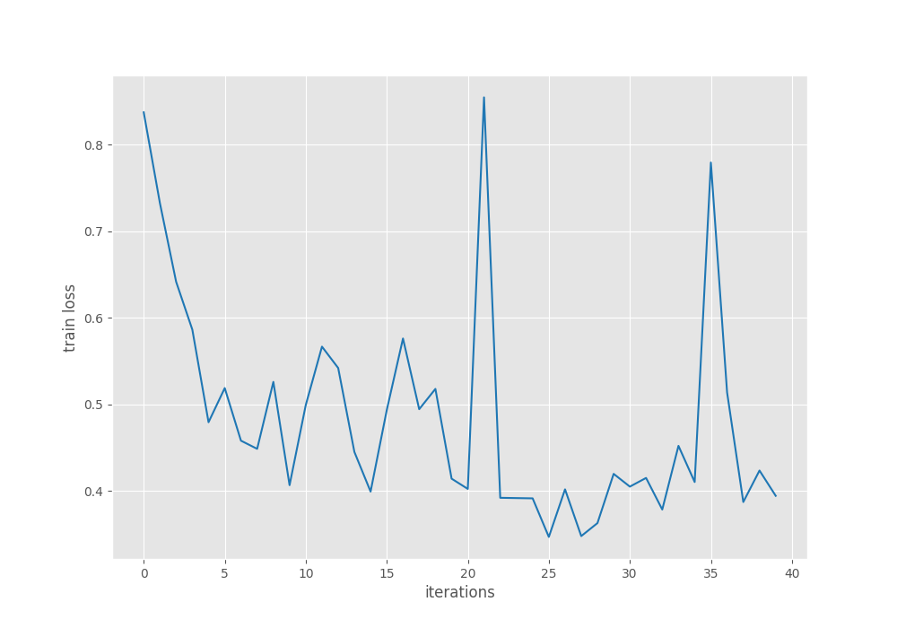
The loss graph seems to fluctuate quite a lot. But then again, the model was able to reach higher mAP values even without the learning rate scheduler.

Mostly, using a learning rate scheduler after 30 epochs will help reduce overfitting.

Evaluation on the Test Set using the Trained PyTorch RetinaNet Model

We also have a held-out test set. Let’s run the evaluation on this test. We can use the eval.py file to do so. This script has the path to the test directory and the best trained weights hard-coded. We just need to execute it.

python eval.py

100%|███████████████████████████████████████████████████████████████████████████████████████████████████████████████████████████████████████████████████████████| 9/9 [00:04<00:00,  1.87it/s]
mAP_50: 86.235
mAP_50_95: 55.253

We reach an mAP of 55.25% at IoU 0.50:0.95 and an mAP of 86.23% at 0.50 IoU.

This is very close to what we got in the best validation loop while training.

Running Inference on the Test Set

To check how many correct detections our custom-trained RetinaNet model is able to make, we can run inference on the test set. Then to get a better idea, we can compare the predictions with the ground truth annotations.

First, let’s run the inference. We will use the inference.py script for this.

python inference.py --input "data/BCCD.v3-raw.voc/test" --threshold 0.3

We just need to provide the directory path to the test folder. The script will run inference on all the images in the directory. Also, we are using a score threshold of 0.3.

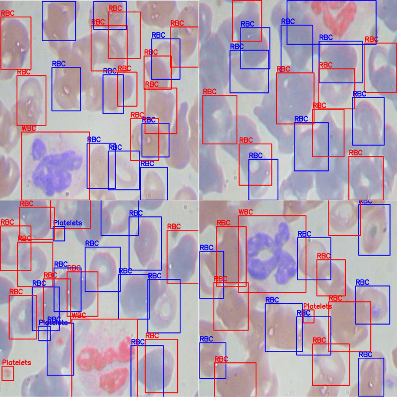
Here are some of the detections along with their ground truth comparison side-by-side.

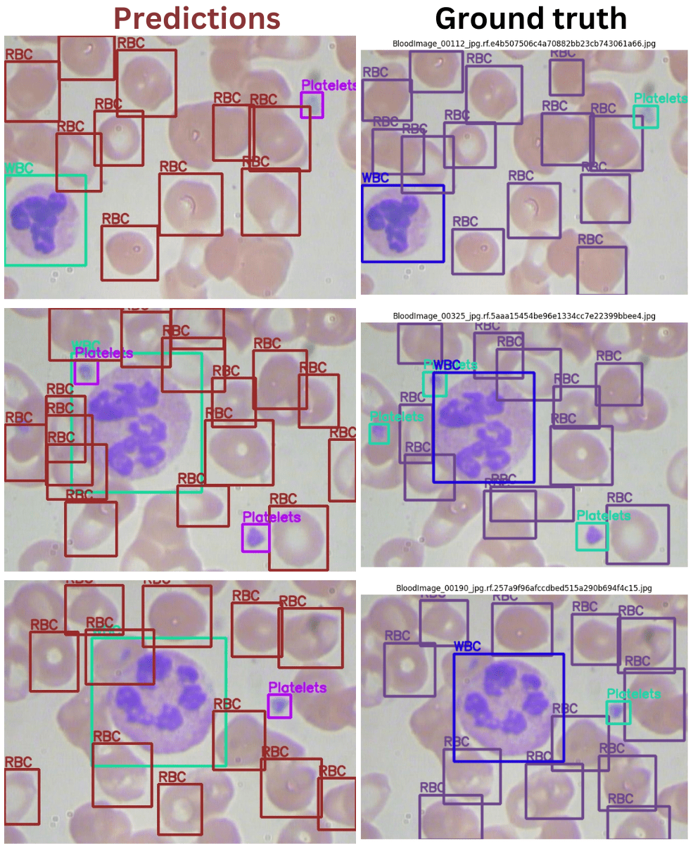
The above results may not be perfect but they are pretty good. Just to think about it, we do not have a very complicated pipeline apart from the dataset preparation. Still, the model was able to learn the features well and the detections are also good.

You can add improvements to this such as collecting more data, adding more augmentations, and adding a scheduling technique as well.

Summary and Conclusion

In this article, we created a simple pipeline to train the PyTorch RetinaNet object detection model. We started with the pretrained Torchvision model and configured it according to our needs. Then we prepared the BCCD dataset and ran training. The results were not perfect but were very good considering the amount of time we spent on the model configuration part. You can take this project further from here and add any improvements that you may want. Or you may just train it on another dataset and see how it performs. I hope that this article was worth your time.

If you any doubts, thoughts, or suggestions, please leave them in the comment section. I will surely address them.

You can contact me using the Contact section. You can also find me on LinkedIn, and Twitter.