Human Action Recognition using 2D CNN with PyTorch

Human action recognition is an important task in computer vision. Starting from real time CCTV surveillance, and sports, to even monitoring drivers in cars, it has a lot of use cases. There are a lot of pretrained models for action recognition. These models are primarily trained on the Kinetics dataset spanning over 100s of classes. But let’s try something different. In this tutorial, we will train a custom action recognition model. We will use a 2D CNN model built using PyTorch and train it for Human Action Recognition.

Just to set the expectations right, we will not be training a huge model. It is going to be a pretrained model and we will fine-tune it. Moreover, the dataset which we will train on does not contain hundreds of classes. This tutorial will act as a proof of concept that fine-tuning a pretrained 2D CNN model can work well enough even when we do not have hundreds of thousands of images. Further, there is another caveat to our approach which is generally not recommended in modern action recognition deep learning models. We will discuss this at the end.

For now, let’s check all the topics that we will cover while training our 2D CNN model for human action recognition.

• First, we will discuss the dataset. This is one of the most important aspects.
• Then we will move on to the coding section. Here, we will create the model, and prepare the dataset, and prepare the training and validation scripts. Next, we will cover the training.
• After training, we will test the trained model on the held-out test set.
• Finally, we will also run inference on unseen videos.

The Human Action Recognition Dataset

In this tutorial, we will use the Human Action Recognition Dataset from Kaggle.

This dataset contains images of human activity and one action class per image. The training set contains 12601 images along with their respective activity class in a CSV file. It also contains a test set with 5410 images. But the test CSV file does not contain the ground truth labels. So, while preparing the dataset, we will split the initial training data into a training and a validation set.

The dataset contains 15 different action classes.

• calling
• clapping
• cycling
• dancing
• drinking
• eating
• fighting
• hugging
• laughing
• listening_to_music
• running
• sitting
• sleeping
• texting
• using_laptop
  

You can go ahead and download the dataset. After extracting it, you should see the following structure.

├── test [5410 entries exceeds filelimit, not opening dir]
├── train [12601 entries exceeds filelimit, not opening dir]
├── Testing_set.csv
└── Training_set.csv

There is a train directory containing all the images and the Training_set.csv file contains the labels for these images. The test directory contains images that we can use for testing the model after training. But the Testing_set.csv file does not contain the ground truth labels. This is because this dataset was part of a competition on the AI Planet website and the Testing_set.csv file was to be used as a submission file.

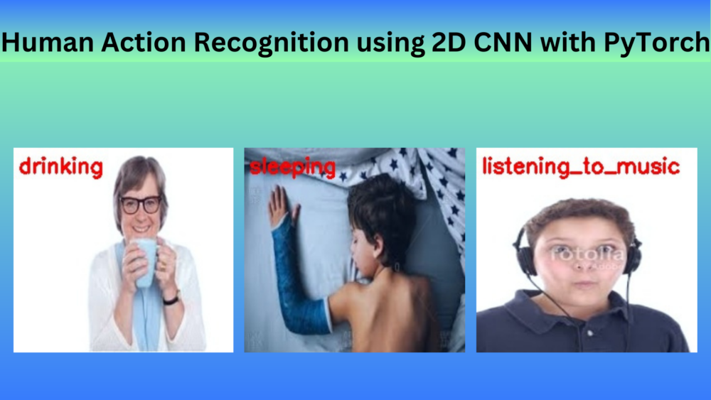
Here are a few images from the training data along with their ground truth classes.

As we can see, the images are quite diverse. Even for the same class, each image is very different.

Project Directory Structure

The following is the directory structure that we are using for the project.

├── input
│   ├── Human Action Recognition
│   └── inference_data
├── outputs
│   ├── inference_results
│   ├── accuracy.png
│   ├── best_model.pth
│   ├── loss.png
│   └── model.pth
└── src
    ├── class_names.py
    ├── datasets.py
    ├── inference.py
    ├── inference_video.py
    ├── model.py
    ├── train.py
    └── utils.py

• The Human Action Recognition directory that we discussed in the previous section resides in the input directory. We also have an inference_data directory containing a few videos that we will carry inference upon after training the model.
• The outputs directory contains all the outputs from training and inference. These include the trained model weights as well.
• Finally, the src directory contains the code file. We have 7 Python files for this project.

You will get access to the trained weights and inference data when downloading the zip file for this post. In case you want to train your own model, please download the dataset from Kaggle.

Human Action Recognition using 2D CNN

From here on, we will start with the coding section of the tutorial. We will go through each of the Python files. However, we will go into the details of the important files only. For the utility scripts, we will keep the explanation sparse.

Download Code

Defining the Class Names

Let’s start with defining the class names in the class_names.py script. This will later on help us with mapping while creating the dataset and also during inference.

class_names = [
    'calling', 
    'clapping', 
    'cycling', 
    'dancing', 
    'drinking', 
    'eating', 
    'fighting', 
    'hugging', 
    'laughing', 
    'listening_to_music', 
    'running', 
    'sitting', 
    'sleeping', 
    'texting', 
    'using_laptop'
]

The Python file simply contains a class_names list with all the labels from the dataset.

Utility and Helper Scripts

While training, we will need functions and classes to save the best model weights and graphs. For that, we will write all the utility code in the utils.py file.

The following block contains the code to save the best model and the final model weights.

import torch
import matplotlib
import matplotlib.pyplot as plt
import os

matplotlib.style.use('ggplot')

class SaveBestModel:
    """
    Class to save the best model while training. If the current epoch's 
    validation loss is less than the previous least less, then save the
    model state.
    """
    def __init__(
        self, best_valid_loss=float('inf')
    ):
        self.best_valid_loss = best_valid_loss
        
    def __call__(
        self, current_valid_loss, epoch, model, out_dir, name
    ):
        if current_valid_loss < self.best_valid_loss:
            self.best_valid_loss = current_valid_loss
            print(f"\nBest validation loss: {self.best_valid_loss}")
            print(f"\nSaving best model for epoch: {epoch+1}\n")
            torch.save({
                'epoch': epoch+1,
                'model_state_dict': model.state_dict(),
                }, os.path.join(out_dir, 'best_'+name+'.pth'))

def save_model(epochs, model, optimizer, criterion, out_dir, name):
    """
    Function to save the trained model to disk.
    """
    torch.save({
                'epoch': epochs,
                'model_state_dict': model.state_dict(),
                'optimizer_state_dict': optimizer.state_dict(),
                'loss': criterion,
                }, os.path.join(out_dir, name+'.pth'))

Upon calling an instance of the SaveBestModel class, it saves the best model based on the loss value. The best weights are defined if the current validation loss is lower than the previous lowest value.

The save_model function simply saves the last weights along with the optimizer state dictionary. We can use this to resume training if we wish to.

We also have a function to save the accuracy and loss plots at the end.

def save_plots(train_acc, valid_acc, train_loss, valid_loss, out_dir):
    """
    Function to save the loss and accuracy plots to disk.
    """
    # Accuracy plots.
    plt.figure(figsize=(10, 7))
    plt.plot(
        train_acc, color='tab:blue', linestyle='-', 
        label='train accuracy'
    )
    plt.plot(
        valid_acc, color='tab:red', linestyle='-', 
        label='validataion accuracy'
    )
    plt.xlabel('Epochs')
    plt.ylabel('Accuracy')
    plt.legend()
    plt.savefig(os.path.join(out_dir, 'accuracy.png'))
    
    # Loss plots.
    plt.figure(figsize=(10, 7))
    plt.plot(
        train_loss, color='tab:blue', linestyle='-', 
        label='train loss'
    )
    plt.plot(
        valid_loss, color='tab:red', linestyle='-', 
        label='validataion loss'
    )
    plt.xlabel('Epochs')
    plt.ylabel('Loss')
    plt.legend()
    plt.savefig(os.path.join(out_dir, 'loss.png'))

The save_plots function simply accepts the lists containing the respective values and saves the plots to disk.

Preparing the Human Action Recognition Dataset for 2D CNN Training

The dataset preparation is going to be very essential in this case. We have a single training dataset which we will need to split to get the validation data. Also, as the ground truth labels are present in a CSV file, we will need to write a custom dataset class for that.

All the code related to dataset preparation goes into the datasets.py file.

Let’s start by defining the import statements and the necessary constants.

import os
import pandas as pd
import cv2

from torchvision import transforms
from torch.utils.data import DataLoader, Dataset

# Required constants.
ROOT_DIR = os.path.join('..', 'input', 'Human Action Recognition', 'train')
CSV_PATH = os.path.join(
    '..', 'input', 'Human Action Recognition', 'Training_set.csv'
)
TRAIN_RATIO = 85
VALID_RATIO = 100 - TRAIN_RATIO
IMAGE_SIZE = 224 # Image size of resize when applying transforms.
NUM_WORKERS = 4 # Number of parallel processes for data preparation.

We will need the transforms module for defining the augmentations and preprocessing. The DataLoader and Dataset classes are necessary for creating the custom dataset class.

We also define the following constants in the above code block:

• ROOT_DIR: This is the path to the root directory containing the images.
• CSV_PATH: The path to the training CSV file.
• TRAIN_RATIO: This is the percentage of the data that we will use for training. It is 85% in our case.
• VALID_RATIO: We will use the rest of the 15% as the validation data.
• IMAGE_SIZE: We will resize all the images to 224×224 dimensions while transforming them.
• NUM_WORKERS: This is the number of workers to use for data loading.

The Training and Validation Transforms

The following two functions define the dataset transforms and augmentations.

# Training transforms
def get_train_transform(image_size):
    train_transform = transforms.Compose([
        transforms.ToPILImage(),
        transforms.Resize((image_size, image_size)),
        transforms.RandomHorizontalFlip(p=0.5),
        transforms.RandomRotation(35),
        transforms.RandomAdjustSharpness(sharpness_factor=2, p=0.5),
        transforms.GaussianBlur(kernel_size=3),
        transforms.RandomGrayscale(p=0.5),
        transforms.RandomRotation(45),
        transforms.RandomAutocontrast(p=0.5),
        transforms.ToTensor(),
        transforms.Normalize(
            mean=[0.485, 0.456, 0.406],
            std=[0.229, 0.224, 0.225]
            )
    ])
    return train_transform

# Validation transforms
def get_valid_transform(image_size):
    valid_transform = transforms.Compose([
        transforms.ToPILImage(),
        transforms.Resize((image_size, image_size)),
        transforms.ToTensor(),
        transforms.Normalize(
            mean=[0.485, 0.456, 0.406],
            std=[0.229, 0.224, 0.225]
            )
    ])
    return valid_transform

The get_train_transform() contains all the augmentations and transforms that we need for the training set. As we can see, we apply quite a lot of augmentations. This is mostly to prevent overfitting and make the model see different images on each epoch. We apply the ImageNet normalizations as we will fine-tune a model pretrained on the ImageNet dataset.

For the validation transforms, we just apply resizing and normalization.

Shuffling the CSV File

After reading the CSV file, we need to ensure that it is shuffled. Because we will map the image names and corresponding labels from the CSV file, it is quite important that we do not use the CSV file without shuffling.

def shuffle_csv():
    df = pd.read_csv(CSV_PATH)
    df = df.sample(frac=1)

    num_train = int(len(df)*(TRAIN_RATIO/100))
    num_valid = int(len(df)*(VALID_RATIO/100))
    
    train_df = df[:num_train].reset_index(drop=True)
    valid_df = df[-num_valid:].reset_index(drop=True)
    return train_df, valid_df

The shuffle_csv() function reads the CSV file, shuffles it, and returns the training and validation dataframes. We can then directly use these dataframes in the custom dataset class.

The Custom Dataset Class

The following code block contains the custom dataset class.

class CustomDataset(Dataset):
    def __init__(self, df, class_names, is_train=False):
        self.image_dir = ROOT_DIR
        self.df = df
        self.image_names = self.df.filename
        self.labels = list(self.df.label)
        self.class_names = class_names
        if is_train:
            self.transform = get_train_transform(IMAGE_SIZE)
        else:
            self.transform = get_valid_transform(IMAGE_SIZE)

    def __len__(self):
        return len(self.image_names)
    
    def __getitem__(self, index):
        image_path = os.path.join(self.image_dir, self.image_names[index])
        label = self.labels[index]
        # Process and transform images.
        image = cv2.imread(image_path)
        image = cv2.cvtColor(image, cv2.COLOR_BGR2RGB)
        image_tensor = self.transform(image)
        class_num = self.class_names.index(label)
        return {
            'image': image_tensor,
            'label': class_num
        }

As we have the dataframes in place, the code becomes simple.

The __init__() method initializes the root directory, the required dataframe, and class names. We also have an is_frame variable which controls the transform applied to the data.

The __getitem__() method reads the image by combining the root directoy path and the image file names from the dataframe. The label variable holds the corresponding label for the image. After converting the image to RGB color format, we apply the appropriate transforms. The method returns a dictionary with an image and label key.

For getting the data loaders, we have simple get_data_loaders function.

def get_data_loaders(dataset_train, dataset_valid, batch_size):
    """
    Prepares the training and validation data loaders.
    :param dataset_train: The training dataset.
    :param dataset_valid: The validation dataset.
    Returns the training and validation data loaders.
    """
    train_loader = DataLoader(
        dataset_train, batch_size=batch_size, 
        shuffle=True, num_workers=NUM_WORKERS
    )
    valid_loader = DataLoader(
        dataset_valid, batch_size=batch_size, 
        shuffle=False, num_workers=NUM_WORKERS
    )
    return train_loader, valid_loader 

This simply accepts the datasets as parameters and returns the respective data loaders.

That’s all we need to prepare the dataset.

Preparing the ResNet50 Model

Earlier we discussed that we will use a 2D CNN model for human activity recognition in this tutorial. Precisely, we will fine-tune a ResNet50 model that has already been pretrained on the ImageNet dataset.

Here is the entire code for the model preparation that is present in the model.py file.

from torchvision import models

import torch.nn as nn

def build_model(fine_tune=True, num_classes=10):
    model = models.resnet50(weights='DEFAULT')
    if fine_tune:
        print('[INFO]: Fine-tuning all layers...')
        for params in model.parameters():
            params.requires_grad = True
    if not fine_tune:
        print('[INFO]: Freezing hidden layers...')
        for params in model.parameters():
            params.requires_grad = False
    model.fc = nn.Linear(in_features=2048, out_features=num_classes, bias=True)
    return model

The model accepts the fine_tune and num_classes as arguments. If we pass fine_tune as True, then all the intermediate layers of the model will be retrained. Else, only the classification head will be trained.

Also, we need to modify the final classification layer of the model according to our number of classes. We can access it through model.fc as we can see in the above code block.

Training Script for Human Action Recognition using 2D CNN

The training script will combine everything that we have covered till now. This is also the executable script that we will run to start the training.

All the code for the training script goes into the train.py file. Let’s start with importing the necessary modules, setting the seed for reproducibility and defining the argument parsers.

import torch
import argparse
import torch.nn as nn
import torch.optim as optim
import os
import numpy as np
import random

from tqdm.auto import tqdm
from model import build_model
from datasets import get_data_loaders, shuffle_csv, CustomDataset
from utils import save_model, save_plots, SaveBestModel
from class_names import class_names

seed = 42
np.random.seed(seed)
random.seed(seed)
torch.manual_seed(seed)
torch.cuda.manual_seed(seed)
torch.cuda.manual_seed_all(seed)
torch.backends.cudnn.deterministic = True

# Construct the argument parser.
parser = argparse.ArgumentParser()
parser.add_argument(
    '-e', '--epochs', 
    type=int, 
    default=10,
    help='Number of epochs to train our network for'
)
parser.add_argument(
    '-lr', '--learning-rate', 
    type=float,
    dest='learning_rate', 
    default=0.001,
    help='Learning rate for training the model'
)
parser.add_argument(
    '-b', '--batch-size',
    dest='batch_size',
    default=32,
    type=int
)
parser.add_argument(
    '-ft', '--fine-tune',
    dest='fine_tune' ,
    action='store_true',
    help='pass this to fine tune all layers'
)
parser.add_argument(
    '--save-name',
    dest='save_name',
    default='model',
    help='file name of the final model to save'
)
parser.add_argument(
    '--scheduler',
    action='store_true',
    help='use learning rate scheduler if passed'
)
args = parser.parse_args()

The training script supports the following command line arguments.

• --epochs: The number of epochs that we want to run the training for.
• --learning-rate: The learning rate for the optimizer.
• --batch-size: This will define the batch size for the data loader.
• --fine-tune: This is a boolean argument indicating whether we want to train all the layers of the model or not.
• --save-name: The file name to save the final model with. By default, it will be saved as model.pth.
• --scheduler: This is also a boolean argument. If we pass this, then a learning rate schedule will be applied after a certain epoch.

The Training and Validation Functions

Next, we have the training and validation functions.

# Training function.
def train(model, trainloader, optimizer, criterion):
    model.train()
    print('Training')
    train_running_loss = 0.0
    train_running_correct = 0
    counter = 0
    prog_bar = tqdm(
        trainloader, 
        total=len(trainloader), 
        bar_format='{l_bar}{bar:20}{r_bar}{bar:-20b}'
    )
    for i, data in enumerate(prog_bar):
        counter += 1
        image, labels = data['image'], data['label']
        image = image.to(device)
        labels = labels.to(device)
        optimizer.zero_grad()
        # Forward pass.
        outputs = model(image)
        # Calculate the loss.
        loss = criterion(outputs, labels)
        train_running_loss += loss.item()
        # Calculate the accuracy.
        _, preds = torch.max(outputs.data, 1)
        train_running_correct += (preds == labels).sum().item()
        # Backpropagation.
        loss.backward()
        # Update the weights.
        optimizer.step()
    
    # Loss and accuracy for the complete epoch.
    epoch_loss = train_running_loss / counter
    epoch_acc = 100. * (train_running_correct / len(trainloader.dataset))
    return epoch_loss, epoch_acc

# Validation function.
def validate(model, testloader, criterion):
    model.eval()
    print('Validation')
    valid_running_loss = 0.0
    valid_running_correct = 0
    counter = 0
    prog_bar = tqdm(
        testloader, 
        total=len(testloader), 
        bar_format='{l_bar}{bar:20}{r_bar}{bar:-20b}'
    )
    with torch.no_grad():
        for i, data in enumerate(prog_bar):
            counter += 1
            
            image, labels = data['image'], data['label']
            image = image.to(device)
            labels = labels.to(device)
            # Forward pass.
            outputs = model(image)
            # Calculate the loss.
            loss = criterion(outputs, labels)
            valid_running_loss += loss.item()
            # Calculate the accuracy.
            _, preds = torch.max(outputs.data, 1)
            valid_running_correct += (preds == labels).sum().item()
        
    # Loss and accuracy for the complete epoch.
    epoch_loss = valid_running_loss / counter
    epoch_acc = 100. * (valid_running_correct / len(testloader.dataset))
    return epoch_loss, epoch_acc

The above functions are very generic PyTorch training and validation functions for image classification.

if __name__ == '__main__':
    # Create a directory with the model name for outputs.
    out_dir = os.path.join('..', 'outputs')
    os.makedirs(out_dir, exist_ok=True)
    # Load the training and validation datasets.
    train_df, valid_df = shuffle_csv()
    dataset_train = CustomDataset(train_df, class_names, is_train=True)
    dataset_valid = CustomDataset(valid_df, class_names, is_train=False)
    print(f"[INFO]: Number of training images: {len(dataset_train)}")
    print(f"[INFO]: Number of validation images: {len(dataset_valid)}")
    print(f"[INFO]: Classes: {class_names}")
    # Load the training and validation data loaders.
    train_loader, valid_loader = get_data_loaders(
        dataset_train, dataset_valid, batch_size=args.batch_size
    )

    # Learning_parameters. 
    lr = args.learning_rate
    epochs = args.epochs
    device = ('cuda' if torch.cuda.is_available() else 'cpu')
    print(f"Computation device: {device}")
    print(f"Learning rate: {lr}")
    print(f"Epochs to train for: {epochs}\n")

    # Load the model.
    model = build_model(
        fine_tune=args.fine_tune, 
        num_classes=len(class_names)
    ).to(device)
    print(model)
    
    # Total parameters and trainable parameters.
    total_params = sum(p.numel() for p in model.parameters())
    print(f"{total_params:,} total parameters.")
    total_trainable_params = sum(
        p.numel() for p in model.parameters() if p.requires_grad)
    print(f"{total_trainable_params:,} training parameters.")

    # Optimizer.
    # optimizer = optim.SGD(
        # model.parameters(), lr=lr, momentum=0.9, nesterov=True
    # )
    optimizer = optim.Adam(model.parameters(), lr=lr)
    # Loss function.
    criterion = nn.CrossEntropyLoss()

    # Initialize `SaveBestModel` class.
    save_best_model = SaveBestModel()

    # LR scheduler.
    scheduler = optim.lr_scheduler.MultiStepLR(
        optimizer, milestones=[7], gamma=0.1, verbose=True
    )

    # Lists to keep track of losses and accuracies.
    train_loss, valid_loss = [], []
    train_acc, valid_acc = [], []
    # Start the training.
    for epoch in range(epochs):
        print(f"[INFO]: Epoch {epoch+1} of {epochs}")
        train_epoch_loss, train_epoch_acc = train(
            model, train_loader, optimizer, criterion
        )
        valid_epoch_loss, valid_epoch_acc = validate(
            model, valid_loader, criterion
        )
        train_loss.append(train_epoch_loss)
        valid_loss.append(valid_epoch_loss)
        train_acc.append(train_epoch_acc)
        valid_acc.append(valid_epoch_acc)
        print(f"Training loss: {train_epoch_loss:.3f}, training acc: {train_epoch_acc:.3f}")
        print(f"Validation loss: {valid_epoch_loss:.3f}, validation acc: {valid_epoch_acc:.3f}")
        save_best_model(
            valid_epoch_loss, epoch, model, out_dir, args.save_name
        )
        if args.scheduler:
            scheduler.step()
        print('-'*50)

    # Save the trained model weights.
    save_model(epochs, model, optimizer, criterion, out_dir, args.save_name)
    # Save the loss and accuracy plots.
    save_plots(train_acc, valid_acc, train_loss, valid_loss, out_dir)
    print('TRAINING COMPLETE')We have the training loop inside the main code block. This part is going to be a bit long.

The above code block assembles everything. It starts by creating the output directory. Then it initializes the datasets, creates the data loaders, builds the model, and defines the optimizer & loss function. We also have a MultiStepLR for the optimizer with a single milestone of 7 epochs. This means that the learning rate will be reduced by a factor of 10 after 7 epochs.

The training loop starts on line 188. We check whether we can save the best model after each epoch using the validation loss. After the training finishes, we save the model with the final weights and the plots for accuracy & loss.

Training the ResNet50 Model

To start the training, you can open the terminal within the src directory and execute the following command.

python train.py --epochs 15 --fine-tune --batch-size 32 -lr 0.0001 --scheduler

We are training the model for 15 epochs with a batch size of 32. The initial learning rate is 0.0001. We are also using the learning rate scheduler. This means that the learning rate will become 0.00001 after 7 epochs.

Here are the shortened outputs from the terminal.

[INFO]: Number of training images: 10710
[INFO]: Number of validation images: 1890
[INFO]: Classes: ['calling', 'clapping', 'cycling', 'dancing', 'drinking', 'eating', 'fighting', 'hugging', 'laughing', 'listening_to_music', 'running', 'sitting', 'sleeping', 'texting', 'using_laptop']
Computation device: cuda
Learning rate: 0.0001
Epochs to train for: 15

[INFO]: Fine-tuning all layers...
.
.
.
Adjusting learning rate of group 0 to 1.0000e-04.
[INFO]: Epoch 1 of 15
Training
100%|████████████████████| 335/335 [00:30<00:00, 10.97it/s]                                                                                                                                   
Validation
100%|████████████████████| 60/60 [00:02<00:00, 26.36it/s]                                                                                                                                     
Training loss: 1.599, training acc: 50.411
Validation loss: 0.841, validation acc: 75.026

Best validation loss: 0.8405184497435888

Saving best model for epoch: 1

Adjusting learning rate of group 0 to 1.0000e-04.
--------------------------------------------------
.
.
.
[INFO]: Epoch 12 of 15
Training
100%|████████████████████| 335/335 [00:29<00:00, 11.31it/s]                                                                                                                                   
Validation
100%|████████████████████| 60/60 [00:02<00:00, 27.89it/s]                                                                                                                                     
Training loss: 0.258, training acc: 91.858
Validation loss: 0.616, validation acc: 82.857

Best validation loss: 0.6160886674954479

Saving best model for epoch: 12

Adjusting learning rate of group 0 to 1.0000e-05.
--------------------------------------------------
.
.
.
[INFO]: Epoch 15 of 15
Training
100%|████████████████████| 335/335 [00:29<00:00, 11.41it/s]                                                                                                                                   
Validation
100%|████████████████████| 60/60 [00:02<00:00, 27.69it/s]                                                                                                                                     
Training loss: 0.230, training acc: 92.932
Validation loss: 0.637, validation acc: 82.698
Adjusting learning rate of group 0 to 1.0000e-05.
--------------------------------------------------
TRAINING COMPLETE

We get the best model on epoch 12. The best validation loss is 0.61 and the best validation accuracy is 82.85%.

Let’s take a look at the loss and accuracy graphs to get some more insights.

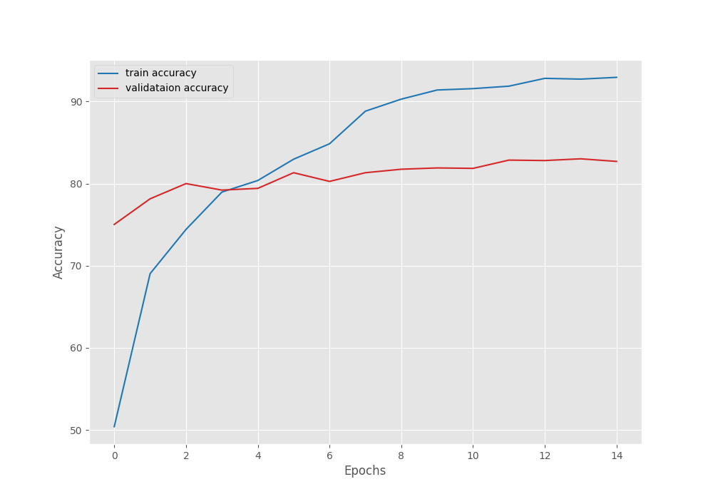
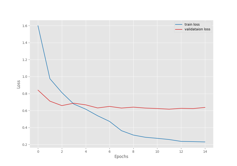
Clearly, reducing the learning rate after 7 epochs helped the validation loss from going up. Also, the validation accuracy kept on increasing. But it seems that the validation loss is again going up after 15 epochs. To continue training, we will need to employ some more regularization techniques.

But for now, we have a trained model.

Inference on Images

The dataset came with a set of test images that we have not used yet. We can use them to run inference and check the performance of the trained model.

Before that, we will go through the inference script and a brief explanation of it. The image inference code is in the inference.py script.

We start with importing the modules, creating the argument parser, and defining the constants for the image size and device.

import torch
import numpy as np
import cv2
import os
import torch.nn.functional as F
import torchvision.transforms as transforms
import glob
import argparse
import pathlib

from model import build_model
from class_names import class_names as CLASS_NAMES

# Construct the argument parser.
parser = argparse.ArgumentParser()
parser.add_argument(
    '-w', '--weights', 
    default='../outputs/best_model.pth',
    help='path to the model weights',
)
args = parser.parse_args()

# Constants and other configurations.
DEVICE = torch.device('cuda:0' if torch.cuda.is_available() else 'cpu')
IMAGE_RESIZE = 224

As we resized the images to 224×224 resolution during training, we will do the same here as well.

Next, we define the transforms and a few helper functions.

# Validation transforms
def get_test_transform(image_size):
    test_transform = transforms.Compose([
        transforms.ToPILImage(),
        transforms.Resize((image_size, image_size)),
        transforms.ToTensor(),
        transforms.Normalize(
            mean=[0.485, 0.456, 0.406],
            std=[0.229, 0.224, 0.225]
        )
    ])
    return test_transform

def denormalize(
    x, 
    mean=[0.485, 0.456, 0.406], 
    std=[0.229, 0.224, 0.225]
):
    for t, m, s in zip(x, mean, std):
        t.mul_(s).add_(m)
    return torch.clamp(x, 0, 1)

def annotate_image(image, output_class):
    image = denormalize(image).cpu()
    image = image.squeeze(0).permute((1, 2, 0)).numpy()
    image = np.ascontiguousarray(image, dtype=np.float32)
    image = cv2.cvtColor(image, cv2.COLOR_RGB2BGR)
    class_name = CLASS_NAMES[int(output_class)]
    cv2.putText(
        image,
        class_name,
        (5, 25),
        cv2.FONT_HERSHEY_SIMPLEX,
        0.7,
        (0, 0, 255),
        2, 
        lineType=cv2.LINE_AA
    )
    return image

def inference(model, testloader, DEVICE):
    """
    Function to run inference.

    :param model: The trained model.
    :param testloader: The test data loader.
    :param DEVICE: The computation device.
    """
    model.eval()
    counter = 0
    with torch.no_grad():
        counter += 1
        image = testloader
        image = image.to(DEVICE)

        # Forward pass.
        outputs = model(image)
    # Softmax probabilities.
    predictions = F.softmax(outputs, dim=1).cpu().numpy()
    # Predicted class number.
    output_class = np.argmax(predictions)
    # Show and save the results.
    result = annotate_image(image, output_class)
    return result

• The denormalize() function denormalizes the transformed images.
• annotate_image() annotates the class name on top of a given image.
• The inference() function does the forward pass of the image tensor through the model.

Then we have the main block.

if __name__ == '__main__':
    weights_path = pathlib.Path(args.weights)
    model_name = str(weights_path).split(os.path.sep)[-2]
    print(model_name)
    infer_result_path = os.path.join(
        '..', 'outputs', 'inference_results', model_name
    )
    os.makedirs(infer_result_path, exist_ok=True)

    checkpoint = torch.load(weights_path)
    # Load the model.
    model = build_model(
        fine_tune=False, 
        num_classes=len(CLASS_NAMES)
    ).to(DEVICE)
    model.load_state_dict(checkpoint['model_state_dict'])

    all_image_paths = glob.glob(
        os.path.join('..', 'input', 'Human Action Recognition', 'test', '*')
    )

    transform = get_test_transform(IMAGE_RESIZE)

    for i, image_path in enumerate(all_image_paths):
        print(f"Inference on image: {i+1}")
        image = cv2.imread(image_path)
        image = cv2.cvtColor(image, cv2.COLOR_BGR2RGB)
        image = transform(image)
        image = torch.unsqueeze(image, 0)
        result = inference(
            model, 
            image,
            DEVICE
        )
        # Save the image to disk.
        image_name = image_path.split(os.path.sep)[-1]
        cv2.imshow('Image', result)
        cv2.waitKey(1)
        cv2.imwrite(
            os.path.join(infer_result_path, image_name), result*255.
        )

After carrying out inference on each image, we save the annotated images to outputs/inference_results/image_outputs directory.

We can execute the following command to carry out inference.

python inference.py

Because we do not have the ground truth of the test images, we need to analyze the results manually. The following figure shows some results where the model predicted the class correctly.

Now, some images where the model could not predict the correct class.

We can see that the model has a lot of room to improve.

Inference on Videos

For some final tests, let’s run inference on unseen videos from the internet. All the code for video inference will go into the inference_video.py script.

A lot of code will remain similar to the image inference script. So, we need not go into a detailed explanation. The following block shows the code till the preparation of the video file and just before we start looping over the frames.

import torch
import cv2
import time
import argparse
import torchvision.transforms as transforms
import pathlib
import os
import torch.nn.functional as F
import numpy as np

from model import build_model
from class_names import class_names as CLASS_NAMES

# construct the argumet parser to parse the command line arguments
parser = argparse.ArgumentParser()
parser.add_argument(
    '-i', '--input', 
    default='input/video_1.mp4', 
    help='path to the input video'
)
parser.add_argument(
    '-w', '--weights', 
    default='../outputs/best_model.pth',
    help='path to the model weights',
)
args = parser.parse_args()

OUT_DIR = '../outputs/inference_results/video_outputs'
os.makedirs(OUT_DIR, exist_ok=True)

# set the computation device
DEVICE = torch.device('cuda:0' if torch.cuda.is_available() else 'cpu')
IMAGE_RESIZE = 224

# Validation transforms
def get_test_transform(image_size):
    test_transform = transforms.Compose([
        transforms.ToPILImage(),
        transforms.Resize((image_size, image_size)),
        transforms.ToTensor(),
        transforms.Normalize(
            mean=[0.485, 0.456, 0.406],
            std=[0.229, 0.224, 0.225]
        )
    ])
    return test_transform
transform = get_test_transform(IMAGE_RESIZE)

weights_path = pathlib.Path(args.weights)
checkpoint = torch.load(weights_path)
# Load the model.
model = build_model(
    fine_tune=False, 
    num_classes=len(CLASS_NAMES)
).to(DEVICE)
model.load_state_dict(checkpoint['model_state_dict'])

cap = cv2.VideoCapture(args.input)
# get the frame width and height
frame_width = int(cap.get(3))
frame_height = int(cap.get(4))
# define the outfile file name
save_name = f"{args.input.split('/')[-1].split('.')[0]}"
# define codec and create VideoWriter object 
out = cv2.VideoWriter(f"{OUT_DIR}/{save_name}.mp4", 
                      cv2.VideoWriter_fourcc(*'mp4v'), 30, 
                      (frame_width, frame_height))
# to count the total number of frames iterated through
frame_count = 0
# to keep adding the frames' FPS
total_fps = 0 

Then, we loop over the frames and forward pass each frame through the model.

while(cap.isOpened()):
    # capture each frame of the video
    ret, frame = cap.read()
    if ret:
        rgb_frame = cv2.cvtColor(frame, cv2.COLOR_BGR2RGB)
        # apply transforms to the input image
        input_tensor = transform(rgb_frame)
        # add the batch dimensionsion
        input_batch = input_tensor.unsqueeze(0) 

        # move the input tensor and model to the computation device
        input_batch = input_batch.to(DEVICE)
        model.to(DEVICE)

        with torch.no_grad():
            start_time = time.time()
            outputs = model(input_batch)
            end_time = time.time()

        # get the softmax probabilities
        probabilities = F.softmax(outputs, dim=1).cpu()
        # get the top 1 prediction
        # top1_prob, top1_catid = torch.topk(probabilities, k=1)
        output_class = np.argmax(probabilities)

        # get the current fps
        fps = 1 / (end_time - start_time)
        # add `fps` to `total_fps`
        total_fps += fps
        # increment frame count
        frame_count += 1
        cv2.putText(frame, f"{fps:.3f} FPS", (15, 30), cv2.FONT_HERSHEY_SIMPLEX,
                        1, (0, 255, 0), 2)
        cv2.putText(frame, f"{CLASS_NAMES[int(output_class)]}", (15, 60), cv2.FONT_HERSHEY_SIMPLEX,
                        1, (0, 255, 0), 2)
        cv2.imshow('Result', frame)
        out.write(frame)
        if cv2.waitKey(1) & 0xFF == ord('q'):
            break
    else:
        break
    
# release VideoCapture()
cap.release()
# close all frames and video windows
cv2.destroyAllWindows()
# calculate and print the average FPS
avg_fps = total_fps / frame_count
print(f"Average FPS: {avg_fps:.3f}")

To start the inference, we need to execute the script and provide the path to an input video.

Starting with an example where a man is talking on the phone.

python inference_video.py --input ../input/inference_data/calling.mp4 

We can see that the model is predicting the calling perfectly here. It is predicting the action as calling in all the frames.

Let’s check some more results before concluding anything.

Here is an example where a person is standing and listening to music.

python inference_video.py --input ../input/inference_data/listening_to_music.mp4

The model predicts the listening_to_music class correctly in a lot of frames. But it is also predicting sitting and calling.

Now, one final video inference.

python inference_video.py --input ../input/inference_data/drinking.mp4

This is very interesting. Whenever the bottle is visible in the frame, the model correctly predicts drinking. As soon as the bottle goes out of frame, it starts to give random output, which is not entirely unexpected as it does not see drinking equipment in the frame.

Further Improvements

From the above experiments, we can conclude that although the model is performing well, we can improve the results a lot.

• Firstly, going through the model. Generally, we should not use 2D convolutional neural network models for action recognition. LSTMs and more recently, 3D CNN models show much more potential.
• Secondly, even if we go with the 2D convolutional neural network model, there is one trick that we can use to improve the inference results. We can take the rolling average prediction. This means that we take the average of K predictions by storing the outputs of K number of frames in a list. Generally, this tends to give better results.

Hopefully, we will cover all these topics in future posts.

Summary and Conclusion

In this tutorial, we trained a 2D CNN model for human action recognition. Starting from preparing the dataset to the inference, we covered all the steps. The results were not perfect but we also discussed how to improve them. Let others know in the comment section in case you build something interesting using the code from this tutorial. I hope this tutorial was worth your time.

If you have any doubts, thoughts, or suggestions, please leave them in the comment section. I will surely address them.

You can contact me using the Contact section. You can also find me on LinkedIn, and Twitter.