Using Custom Backbone for PyTorch SSD for Object Detection

Sovit Ranjan Rath June 5, 2023 18 Comments

A lot of times, the pretrained models out there may not serve our purpose for the problem that we have at hand. In deep learning, one may face this issue with pretrained object detection models quite a lot. For instance, Torchvision has two SSD models pretrained on the COCO dataset. One with VGG16 backbone, and a lite version with MobileNetV3 backbone. But what if we want to change the backbone with a more efficient one? Like ResNet or maybe ShuffleNet. In this tutorial, we will learn how to use a Torchvision ImageNet pretrained custom backbone for PyTorch SSD.

Figure 1. Example output for person detection using PyTorch SSD with custom backbone.

One question that may arise is “Why do we need a custom backbone for an object detection model when we have so so many out there”?

A lot of times, the pretrained models may not suffice our needs. Sometimes, while solving a problem we may not want to use another object detection library apart from PyTorch. Or maybe we do not want to use SSD with VGG16 backbone. Or if nothing else, for learning purposes, so that we can solve any type of object detection problem in the future.

The above reasons are not exhaustive but they are enough to explore how to use a custom backbone for PyTorch SSD models.

Let’s take a look at the points that we will cover in this post.

We will start with a discussion of the dataset.
Then in the coding section, we will primarily focus on the model preparation part. That is, how to load an ImageNet pretrained backbone and attach an SSD object detection head to it.
We will go through the rest of the code as and when required.
After training, we will also run inference on unseen data.

The Person Detection Dataset to Train PyTorch SSD with Custom Backbone

In this tutorial, we will use a fairly simple object detection dataset to train the custom Single Shot Detector. We will train it on a person detection dataset which is easy, to begin with. The model will use a pretrained backbone but it has not learned to detect any objects. So, giving it a simple class to learn will be a good idea.

The dataset that we will use here is a modification of the Pedestrian Detection dataset from Kaggle. The original dataset has some labeling issues.

I have corrected all the labels and you can find the new Person Detection dataset on Kaggle. The annotations are in XML format. All the persons in the images are labeled with person class. The dataset contains 944 training, 160 validation, and 235 test samples.

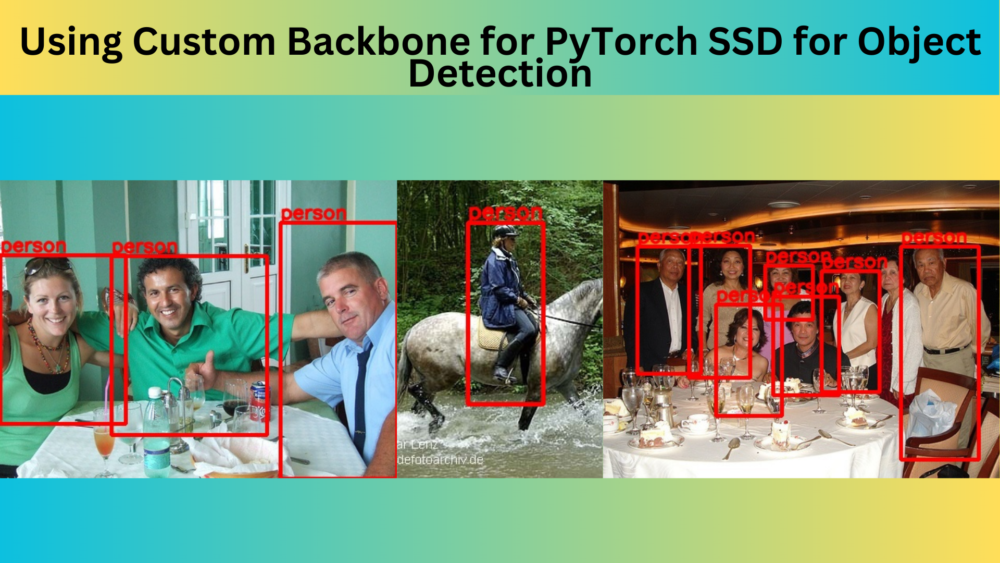
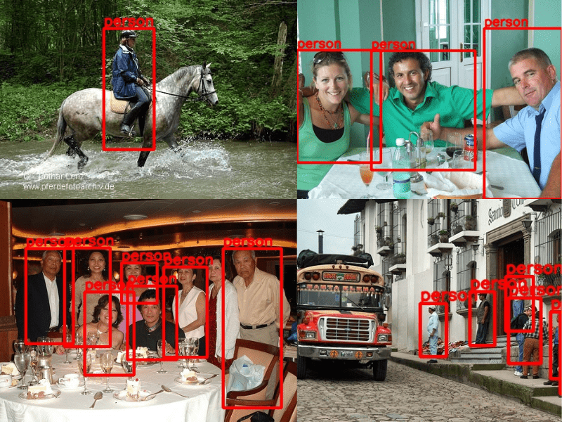
Here are some of the ground truth images from the dataset.

Figure 2. Ground truth images from the person detection dataset to train the PyTorch SSD model.

We can see that the images are present in varied environments. The model, of course, will get to see different people in different scenarios. Hopefully, after training, it will detect a person well on unseen images.

For now, please go ahead and download the dataset if you wish to run the training on your own. After downloading and extracting the dataset, you should see the following structure.

├── Test
│   └── Test
│       └── JPEGImages [470 entries exceeds filelimit, not opening dir]
├── Train
│   └── Train
│       └── JPEGImages [1888 entries exceeds filelimit, not opening dir]
└── Val
    └── Val
        └── JPEGImages [320 entries exceeds filelimit, not opening dir]

After extracting the dataset, we have three directories/subdirectories.

The Train, Val, and Test directories contain the training, validation, and test splits respectively. The images and their corresponding XML annotation files are present inside the JPEGImages directories. You may explore the dataset a bit on your own before moving forward.

The Project Directory Structure

Let’s take a look at the entire directory structure before moving forward with training the Single Shot Detection model with a custom backbone.

├── data
│   ├── inference_data
│   │   ├── image_1.jpg
│   │   ...
│   │   ├── image_4.jpg
│   │   └── video_1.mp4
│   ├── Test
│   │   └── Test
│   │       └── JPEGImages [470 entries exceeds filelimit, not opening dir]
│   ├── Train
│   │   └── Train
│   │       └── JPEGImages [1888 entries exceeds filelimit, not opening dir]
│   └── Val
│       └── Val
│           └── JPEGImages [320 entries exceeds filelimit, not opening dir]
├── inference_outputs
│   ├── images [239 entries exceeds filelimit, not opening dir]
│   └── videos
│       └── video_1.mp4
├── notebooks
│   └── visualizations_data.ipynb
├── outputs
│   ├── best_model.pth
│   ├── last_model.pth
│   ├── map.png
│   └── train_loss.png
├── config.py
├── custom_utils.py
├── datasets.py
├── eval.py
├── inference.py
├── inference_video.py
├── model.py
└── train.py

First, we have the data directory. This contains the person dataset in the Train, Val, and Test folders as discussed earlier. Along with that, we also have an inference_data directory containing some images and videos. We will use these for inference after training the model.
Second, we have the inference_outputs and outputs directories. These contain the outputs from the inference and training experiments respectively. The training experiment will output the mAP and loss plots along with the trained SSD model.
Third, we have a notebooks directory which we can use for data exploration and visualization.
Finally, directly inside the parent project directory, we have all the Python files. We will mostly focus on the model.py script.

The best trained weights and the inference data will be available via the downloadable zip file that comes with this post. You can directly use them for inference. If you wish to run the training experiments as well, please download the dataset from Kaggle.

Training PyTorch SSD Model with Custom Backbone

In the following coding and training sections, we will mostly focus on the model preparation and dataset preparation part. For other coding sections, we will only have an overview of the most important parts. The downloaded file contains all the scripts. Feel free to take your time and explore the code before your move forward.

Download Code

Download the Source Code for this Tutorial

The Configuration File

We will go through the configuration file first. This defines all the essential components that we need for training and dataset preparation. Going through it will make the exploration of the other parts easier. All the training and dataset configuration goes into the config.py file.

import torch

BATCH_SIZE = 16 # Increase / decrease according to GPU memeory.
RESIZE_TO = 640 # Resize the image for training and transforms.
NUM_EPOCHS = 75 # Number of epochs to train for.
NUM_WORKERS = 4 # Number of parallel workers for data loading.

DEVICE = torch.device('cuda') if torch.cuda.is_available() else torch.device('cpu')

# Training images and XML files directory.
TRAIN_DIR = 'data/Train/Train/JPEGImages'
# Validation images and XML files directory.
VALID_DIR = 'data/Val/Val/JPEGImages'

# Classes: 0 index is reserved for background.
CLASSES = [
    '__background__', 'person'
]

NUM_CLASSES = len(CLASSES)

# Whether to visualize images after crearing the data loaders.
VISUALIZE_TRANSFORMED_IMAGES = False

# Location to save model and plots.
OUT_DIR = 'outputs'

We start with defining the batch size for the data loaders, the image resolution to resize to, the number of epochs to train for, and the number of workers.

Although, we are using an SSD300 model, still, we will resize all images to 640×640 resolution for better performance.

Then we provide the paths to the training and validation directories where the images and annotations reside.

CLASSES contains two classes. One is __background__ and the other is person (the object class from the dataset).

We also have a VISUALIZE_TRANSFORMED_IMAGES attribute. If True, a few transformed images (from the dataloader) will show up on the screen when executing the training script. This helps in debugging and checking if all the augmentations and annotations are correct or not.

PyTorch SSD with ResNet Backbone

We will customize the PyTorch Single Shot Detection model with an ImageNet pretrained backbone. As a starting point, we will use the ResNet34 ImageNet pretrained model. That will help the model to start with some already learned features. The architecture is going to change a bit on top of that when we add the classification and regression heads to the model.

Let’s take a look at the code and then getting into the details will make the custom PyTorch SSD explanation a bit easier. The code for the PyTorch SSD model with the custom backbone resides in the model.py file.

import torchvision
import torch.nn as nn

from torchvision.models.detection.ssd import (
    SSD, 
    DefaultBoxGenerator,
    SSDHead
)

def create_model(num_classes=91, size=300, nms=0.45):
    model_backbone = torchvision.models.resnet34(
        weights=torchvision.models.ResNet34_Weights.DEFAULT
    )
    conv1 = model_backbone.conv1
    bn1 = model_backbone.bn1
    relu = model_backbone.relu
    max_pool = model_backbone.maxpool
    layer1 = model_backbone.layer1
    layer2 = model_backbone.layer2
    layer3 = model_backbone.layer3
    layer4 = model_backbone.layer4
    backbone = nn.Sequential(
        conv1, bn1, relu, max_pool, 
        layer1, layer2, layer3, layer4
    )
    out_channels = [512, 512, 512, 512, 512, 512]
    anchor_generator = DefaultBoxGenerator(
        [[2], [2, 3], [2, 3], [2, 3], [2], [2]],
    )
    num_anchors = anchor_generator.num_anchors_per_location()
    head = SSDHead(out_channels, num_anchors, num_classes)
    model = SSD(
        backbone=backbone,
        num_classes=num_classes,
        anchor_generator=anchor_generator,
        size=(size, size),
        head=head,
        nms_thresh=nms
    )
    return model

Code Explanation for PyTorch SSD with ResNet34 Backbone

First, we import all the necessary classes from torchvision.models.detection.ssd (line 4). After that, all the logic takes place in the create_model function.

On line 11, we create an instance of the ResNet34 model with ImageNet pretrained weights. From lines 14 to 21 we extract all the necessary layers that we need to create the entire backbone before the classification head. Then on line 22, we create the final backbone wrapped within a Sequential module.

After the backbone, we also need to add new convolutional layers for the classification and regression head. The number of layers in both heads has to match. For this, we create an out_channels list on line 26. This defines the input channels of six new 2D convolutional layers. The first input channel in this list has to match the output channel of the last layer from the backbone. This is 512 for ResNet34. For the rest five 2D convolutional layers, we use 512 input channels as well.

Then we define the aspect ratios of anchor boxes using DefaultBoxGenerator. We keep this the same as in the official code that is used for pretraining the model on the COCO dataset. These may not be the best numbers for person detection, but they should work optimally well.

Line 30 defines the number of anchors based on the aspect ratios.

Next, we create the detection and classification head based on out_channels list, num_anchors, and the num_classes.

Note: The number of classes is 2 for this dataset. 0 for the background class, and 1 for the person class.

Finally, we combine all and create the SSD model. We also pass the size argument. According to this, all the images will be resized internally.

The following is the output for the detection and the classification head.

  (head): SSDHead(
    (classification_head): SSDClassificationHead(
      (module_list): ModuleList(
        (0): Conv2d(512, 8, kernel_size=(3, 3), stride=(1, 1), padding=(1, 1))
        (1): Conv2d(512, 12, kernel_size=(3, 3), stride=(1, 1), padding=(1, 1))
        (2): Conv2d(512, 12, kernel_size=(3, 3), stride=(1, 1), padding=(1, 1))
        (3): Conv2d(512, 12, kernel_size=(3, 3), stride=(1, 1), padding=(1, 1))
        (4): Conv2d(512, 8, kernel_size=(3, 3), stride=(1, 1), padding=(1, 1))
        (5): Conv2d(512, 8, kernel_size=(3, 3), stride=(1, 1), padding=(1, 1))
      )
    )
    (regression_head): SSDRegressionHead(
      (module_list): ModuleList(
        (0): Conv2d(512, 16, kernel_size=(3, 3), stride=(1, 1), padding=(1, 1))
        (1): Conv2d(512, 24, kernel_size=(3, 3), stride=(1, 1), padding=(1, 1))
        (2): Conv2d(512, 24, kernel_size=(3, 3), stride=(1, 1), padding=(1, 1))
        (3): Conv2d(512, 24, kernel_size=(3, 3), stride=(1, 1), padding=(1, 1))
        (4): Conv2d(512, 16, kernel_size=(3, 3), stride=(1, 1), padding=(1, 1))
        (5): Conv2d(512, 16, kernel_size=(3, 3), stride=(1, 1), padding=(1, 1))
      )
    )
  )

As we can see, there are 6 convolutional layers in each SSD head.

Custom Utilities and Dataset Preparation

The custom_utils.py script contains a lot of helper functions and classes.

Apart from functions for saving the best model weights and plots, it also contains the augmentations that we apply to the images. We define the augmentations under the get_train_transform() function. These are directly used in the datasets.py script when preparing the dataset.

To prevent overfitting, we apply quite a number of augmentations. Here is a complete list of them.

HorizontalFlip
Blur
MotionBlur
MedianBlur
ToGray
RandomBrightnessContrast
ColorJitter
RandomGamma

We can execute the datasets.py script which shows a few images after decoding them from the data loaders. This way we can verify whether the augmentation and resizing operations are properly applied or not. The following are a few images after executing datasets.py.

Figure 3. Augmented images from the dataloader to train the PyTorch SSD model.

We can see that the images are resized. Also, the first image appears blurry and pixelated because of the augmentations.

The Training Script

The train.py file is the driver script and contains all the code for training. These include the training & validation functions, creating the data loaders, and initializing the model.

We will be using the SGD optimizer with a starting learning rate of 0.0005 and a momentum of 0.9. A learning rate scheduler will be applied after 45 epochs to reduce it by a factor of 10.

If you wish, you can go over the training script before executing the training.

In the parent project directory, execute the following command to start the training.

python train.py

Here is the truncated output from the terminal.

Number of training samples: 944
Number of validation samples: 160
.
.
.
EPOCH 1 of 75
Training
Loss: 9.3790: 100%|███████████████████████████████████████████████████████████████████████████████████████████████████████████████████████████████████████████| 59/59 [00:16<00:00,  3.48it/s]
Validating
100%|█████████████████████████████████████████████████████████████████████████████████████████████████████████████████████████████████████████████████████████| 10/10 [00:01<00:00,  5.18it/s]
Epoch #1 train loss: 12.464
Epoch #1 [email protected]:0.95: 0.036912836134433746
Epoch #1 [email protected]: 0.16292478144168854
Took 0.472 minutes for epoch 0

BEST VALIDATION mAP: 0.036912836134433746

SAVING BEST MODEL FOR EPOCH: 1

SAVING PLOTS COMPLETE...
Adjusting learning rate of group 0 to 5.0000e-04.
.
.
.
EPOCH 37 of 75
Training
Loss: 1.5863: 100%|███████████████████████████████████████████████████████████████████████████████████████████████████████████████████████████████████████████| 59/59 [00:14<00:00,  4.03it/s]
Validating
100%|█████████████████████████████████████████████████████████████████████████████████████████████████████████████████████████████████████████████████████████| 10/10 [00:02<00:00,  4.99it/s]
Epoch #37 train loss: 1.992
Epoch #37 [email protected]:0.95: 0.24836641550064087
Epoch #37 [email protected]: 0.652535080909729
Took 0.360 minutes for epoch 36

BEST VALIDATION mAP: 0.24836641550064087

SAVING BEST MODEL FOR EPOCH: 37

SAVING PLOTS COMPLETE...
Adjusting learning rate of group 0 to 5.0000e-04.
.
.
.
EPOCH 75 of 75
Training
Loss: 0.6868: 100%|███████████████████████████████████████████████████████████████████████████████████████████████████████████████████████████████████████████| 59/59 [00:14<00:00,  3.96it/s]
Validating
100%|█████████████████████████████████████████████████████████████████████████████████████████████████████████████████████████████████████████████████████████| 10/10 [00:01<00:00,  5.12it/s]
Epoch #75 train loss: 0.778
Epoch #75 [email protected]:0.95: 0.22010944783687592
Epoch #75 [email protected]: 0.6166431903839111
Took 0.308 minutes for epoch 74
SAVING PLOTS COMPLETE...
Adjusting learning rate of group 0 to 5.0000e-05.

We use mAP as the object detection evaluation metric here. The model reaches the best mAP of 24.83% at 0.50 IoU on epoch 37. At IoU 0.50:095, the mAP is 65.35%. It is not too bad considering we do not even have 1000 images.

Let’s take a look at the plots.

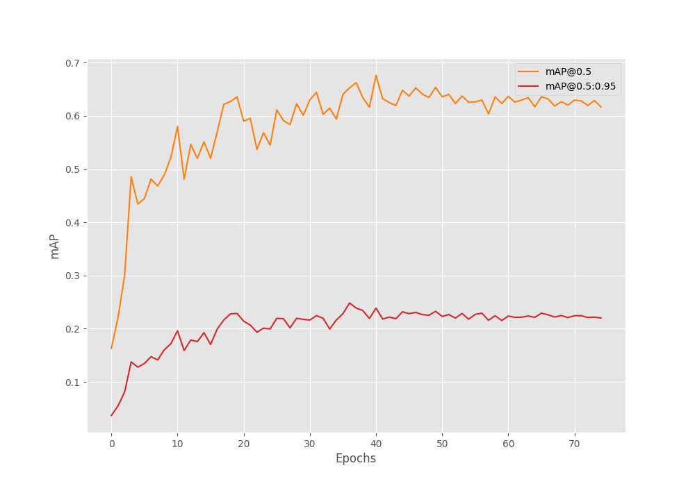
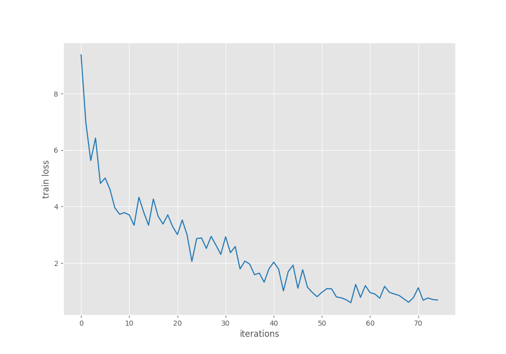
Figure 4. mAP graph after training the PyTorch SSD model with custom backbone on the person detection dataset.

Figure 5. Loss graph after training the PyTorch SSD model with custom backbone on the person detection dataset.

Although the training loss is decreasing till the end of the training, the mAP seems to reduce after around 50 epochs. The mAP does not improve after epoch 37 even after applying the learning rate scheduler.

Evaluation on the Test Dataset

We have the best trained model now. There is also a test set that contains the ground truth annotations. Let’s run evaluation on it using the eval.py script. The directory path has been hardcoded into the script for now.

python eval.py

The following are the results.

100%|████████████████████████████████████████████████████| 15/15 [00:03<00:00,  5.00it/s]
mAP_50: 58.024
mAP_50_95: 19.222

We have an mAP of 58% at 0.50 IoU and 19.22 % at 0.50:0.95 IoU. This is slightly lower compared to the validation set.

Inference on Images and Videos

First, we will run inference on the test images, and then inference on some videos that are not part of the dataset.

To run inference on the test images, we can run the following command:

python inference.py --input data/Test/Test/JPEGImages/

We run inference on all the images from the test set.

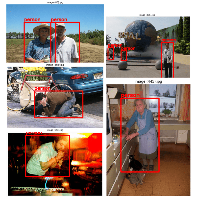
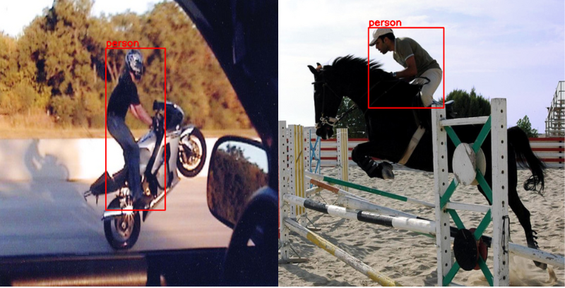
Here are some of the good results.

Some good inference results after training the model. — Figure 6. Some good inference results after training the PyTorch SSD model with custom backbone.

And here are some images where the model did not perform very well.

Figure 7. Some of the bad inference results after training the SSD model.

To run inference on videos, we need to run the inference_video.py script while providing the path to the video file. We use the default score threshold of 0.25 in the following experiments.

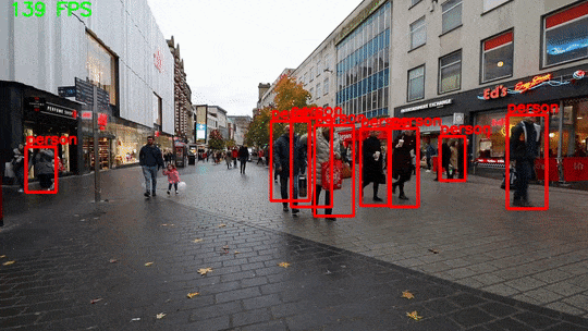
Let’s start with a slightly crowded scene.

python inference_video.py --input data/inference_data/video_1.mp4 --imgsz 640

The model ran at 150 FPS on average on an RTX 3080 GPU.

Clip 1. Inference on a crowded video using the trained PyTorch SSD model with custom ResNet34 backbone.

The results are very mixed here. In some of the frames, the model is performing really well, while in others there is a lot of flickering. Also, it is unable to detect persons at a distance.

Here is another result.

Clip 2. Detection of person who are closer using the PyTorch SSD model with custom backbone.

Interestingly, although the persons are closer to the camera, the flickering does not go away.

Making Improvements to the PyTorch SSD Model with Custom Backbone

There are a few ways to make the model even better.

We can start by training it on more data.
We can also try a larger backbone like ResNet50 which may prove to be a better feature extractor.
Also, we can add FPN (Feature Pyramid Network) which can help the backbone a lot when dealing with small objects.

Posts Not to Miss

Summary and Conclusion

In this tutorial, we learned how to add a custom backbone to a PyTorch SSD head. Using such methods we can create our custom object detection models. We also trained the custom SSD model on a person detection dataset and analyzed the results. Although the results were not very good, they were still decent. We also discussed how to improve the performance of the model further.

If you have any doubts, thoughts, or suggestion, please leave them in the comment section. I will surely address them

You can contact me using the Contact section. You can also find me on LinkedIn, and Twitter.

References

Liked it? Take a second to support Sovit Ranjan Rath on Patreon!

Deep Learning Object Detection PyTorch SSD PyTorch SSD Custom Backbone PyTorch SSD ResNet backbone PyTorch SSD ResNet34 backbone SSD SSD Person Detection

18 thoughts on “Using Custom Backbone for PyTorch SSD for Object Detection”

Ilia says:

July 29, 2023 at 1:51 am

Thank you very much for a great tutorial and providing a code, but I would like to ask a question. I have one issue that I can train a model only for 640×640 resolution. As a dataset I took COCO dataset and chose one class – cars. So when I start training on 1920×1080 for example, after 25 epochs my loss become inf. I tried to reduce learning rate down to 1e-7, changed SGD to Adam, change batch size, tried gradient clipping, but nothing helped. Did you have this issue, how did you resolve it?
Thanks in advance,
Ilia

Reply
1. Sovit Ranjan Rath says:
  
  July 29, 2023 at 8:57 am
  
  Hello Ilia.
  I have not tried with 1920×1080 images. Can you let me know where you are defining the image size?
  According to the config file shown in this post, the images are resized to a square shape. So, did you modify the code to run the training on 1920×1080 images?
  Also, you mention that the loss becomes infinity after 25 epochs. Are the models saved before that epoch able to give proper inference results?
  
  Reply
  1. Annie says:
    
    November 15, 2023 at 8:30 am
    
    Hello Sovit, could you please contact me I need your help regarding my project.?
    
    Reply
Ilia says:

July 30, 2023 at 12:48 am

Hello Sovit, thank you for your reply.
Indeed, in the code there is only one parameter responsible for size, but in model.py in a function “create_model” you can rewrite a line “model=SSD(…, size=(size, size), …)” with “model=SSD(…, size=(1920, 1080), …)”. With batch_size=1 loss become inf after 10 epochs.
And after that I tried image size = 300 (so now image size is a square and in this test I modified config.py only) and again at 11th epoch a loss bacame inf. Here there is a log:
********************************************************************
EPOCH 11 of 75
Training
Loss: 7.0678: 1%|█▎ | 6/766 [00:00<01:30, 8.43it/s]/home/user/.pyenv/versions/3.11.4/lib/python3.11/site-packages/albumentations/augmentations/functional.py:825: RuntimeWarning: invalid value encountered in power
img = np.power(img, gamma)
Loss: inf: 100%|█████████████████████████████████████████████████████████| 766/766 [00:32<00:00, 23.69it/s]
Validating
100%|██████████████████████████████████████████████████████████████████████| 34/34 [00:01<00:00, 18.21it/s]
Epoch #11 train loss: inf
Epoch #11 [email protected]:0.95: 0.0
Epoch #11 [email protected]: 0.0
Took 0.614 minutes for epoch 10
SAVING PLOTS COMPLETE…
Adjusting learning rate of group 0 to 5.0000e-05.
********************************************************************
And whatever I tried, it always failed on 11th epoch for image resolution = 300. And of course on inference the result is very poor because after 10 epochs mAP is about 0.001.

Reply
1. Sovit Ranjan Rath says:
  
  July 30, 2023 at 8:13 pm
  
  Can you try with 300, 300 but with higher batch size? Maybe batch size 1 is causing issues.
  
  Reply
  1. Ilia says:
    
    July 31, 2023 at 2:19 am
    
    Thank you, I will try to vary this and other parameters.
    
    Reply
Adithya Hegde Kota says:

November 10, 2023 at 2:05 pm

umber of training samples: 6236
Number of validation samples: 1557

SSD(
(backbone): Sequential(
(0): Conv2d(3, 64, kernel_size=(7, 7), stride=(2, 2), padding=(3, 3), bias=False)
(1): BatchNorm2d(64, eps=1e-05, momentum=0.1, affine=True, track_running_stats=True)
(2): ReLU(inplace=True)
(3): MaxPool2d(kernel_size=3, stride=2, padding=1, dilation=1, ceil_mode=False)
(4): Sequential(
(0): Bottleneck(
(conv1): Conv2d(64, 64, kernel_size=(1, 1), stride=(1, 1), bias=False)
(bn1): BatchNorm2d(64, eps=1e-05, momentum=0.1, affine=True, track_running_stats=True)
(conv2): Conv2d(64, 64, kernel_size=(3, 3), stride=(1, 1), padding=(1, 1), bias=False)
(bn2): BatchNorm2d(64, eps=1e-05, momentum=0.1, affine=True, track_running_stats=True)
(conv3): Conv2d(64, 256, kernel_size=(1, 1), stride=(1, 1), bias=False)
(bn3): BatchNorm2d(256, eps=1e-05, momentum=0.1, affine=True, track_running_stats=True)
(relu): ReLU(inplace=True)
(downsample): Sequential(
(0): Conv2d(64, 256, kernel_size=(1, 1), stride=(1, 1), bias=False)
(1): BatchNorm2d(256, eps=1e-05, momentum=0.1, affine=True, track_running_stats=True)
)
)
(1): Bottleneck(
(conv1): Conv2d(256, 64, kernel_size=(1, 1), stride=(1, 1), bias=False)
(bn1): BatchNorm2d(64, eps=1e-05, momentum=0.1, affine=True, track_running_stats=True)
(conv2): Conv2d(64, 64, kernel_size=(3, 3), stride=(1, 1), padding=(1, 1), bias=False)
(bn2): BatchNorm2d(64, eps=1e-05, momentum=0.1, affine=True, track_running_stats=True)
(conv3): Conv2d(64, 256, kernel_size=(1, 1), stride=(1, 1), bias=False)
(bn3): BatchNorm2d(256, eps=1e-05, momentum=0.1, affine=True, track_running_stats=True)
(relu): ReLU(inplace=True)
)
(2): Bottleneck(
(conv1): Conv2d(256, 64, kernel_size=(1, 1), stride=(1, 1), bias=False)
(bn1): BatchNorm2d(64, eps=1e-05, momentum=0.1, affine=True, track_running_stats=True)
(conv2): Conv2d(64, 64, kernel_size=(3, 3), stride=(1, 1), padding=(1, 1), bias=False)
(bn2): BatchNorm2d(64, eps=1e-05, momentum=0.1, affine=True, track_running_stats=True)
(conv3): Conv2d(64, 256, kernel_size=(1, 1), stride=(1, 1), bias=False)
(bn3): BatchNorm2d(256, eps=1e-05, momentum=0.1, affine=True, track_running_stats=True)
(relu): ReLU(inplace=True)
)
)
(5): Sequential(
(0): Bottleneck(
(conv1): Conv2d(256, 128, kernel_size=(1, 1), stride=(1, 1), bias=False)
(bn1): BatchNorm2d(128, eps=1e-05, momentum=0.1, affine=True, track_running_stats=True)
(conv2): Conv2d(128, 128, kernel_size=(3, 3), stride=(2, 2), padding=(1, 1), bias=False)
(bn2): BatchNorm2d(128, eps=1e-05, momentum=0.1, affine=True, track_running_stats=True)
(conv3): Conv2d(128, 512, kernel_size=(1, 1), stride=(1, 1), bias=False)
(bn3): BatchNorm2d(512, eps=1e-05, momentum=0.1, affine=True, track_running_stats=True)
(relu): ReLU(inplace=True)
(downsample): Sequential(
(0): Conv2d(256, 512, kernel_size=(1, 1), stride=(2, 2), bias=False)
(1): BatchNorm2d(512, eps=1e-05, momentum=0.1, affine=True, track_running_stats=True)
)
)
(1): Bottleneck(
(conv1): Conv2d(512, 128, kernel_size=(1, 1), stride=(1, 1), bias=False)
(bn1): BatchNorm2d(128, eps=1e-05, momentum=0.1, affine=True, track_running_stats=True)
(conv2): Conv2d(128, 128, kernel_size=(3, 3), stride=(1, 1), padding=(1, 1), bias=False)
(bn2): BatchNorm2d(128, eps=1e-05, momentum=0.1, affine=True, track_running_stats=True)
(conv3): Conv2d(128, 512, kernel_size=(1, 1), stride=(1, 1), bias=False)
(bn3): BatchNorm2d(512, eps=1e-05, momentum=0.1, affine=True, track_running_stats=True)
(relu): ReLU(inplace=True)
)
(2): Bottleneck(
(conv1): Conv2d(512, 128, kernel_size=(1, 1), stride=(1, 1), bias=False)
(bn1): BatchNorm2d(128, eps=1e-05, momentum=0.1, affine=True, track_running_stats=True)
(conv2): Conv2d(128, 128, kernel_size=(3, 3), stride=(1, 1), padding=(1, 1), bias=False)
(bn2): BatchNorm2d(128, eps=1e-05, momentum=0.1, affine=True, track_running_stats=True)
(conv3): Conv2d(128, 512, kernel_size=(1, 1), stride=(1, 1), bias=False)
(bn3): BatchNorm2d(512, eps=1e-05, momentum=0.1, affine=True, track_running_stats=True)
(relu): ReLU(inplace=True)
)
(3): Bottleneck(
(conv1): Conv2d(512, 128, kernel_size=(1, 1), stride=(1, 1), bias=False)
(bn1): BatchNorm2d(128, eps=1e-05, momentum=0.1, affine=True, track_running_stats=True)
(conv2): Conv2d(128, 128, kernel_size=(3, 3), stride=(1, 1), padding=(1, 1), bias=False)
(bn2): BatchNorm2d(128, eps=1e-05, momentum=0.1, affine=True, track_running_stats=True)
(conv3): Conv2d(128, 512, kernel_size=(1, 1), stride=(1, 1), bias=False)
(bn3): BatchNorm2d(512, eps=1e-05, momentum=0.1, affine=True, track_running_stats=True)
(relu): ReLU(inplace=True)
)
)
(6): Sequential(
(0): Bottleneck(
(conv1): Conv2d(512, 256, kernel_size=(1, 1), stride=(1, 1), bias=False)
(bn1): BatchNorm2d(256, eps=1e-05, momentum=0.1, affine=True, track_running_stats=True)
(conv2): Conv2d(256, 256, kernel_size=(3, 3), stride=(2, 2), padding=(1, 1), bias=False)
(bn2): BatchNorm2d(256, eps=1e-05, momentum=0.1, affine=True, track_running_stats=True)
(conv3): Conv2d(256, 1024, kernel_size=(1, 1), stride=(1, 1), bias=False)
(bn3): BatchNorm2d(1024, eps=1e-05, momentum=0.1, affine=True, track_running_stats=True)
(relu): ReLU(inplace=True)
(downsample): Sequential(
(0): Conv2d(512, 1024, kernel_size=(1, 1), stride=(2, 2), bias=False)
(1): BatchNorm2d(1024, eps=1e-05, momentum=0.1, affine=True, track_running_stats=True)
)
)
(1): Bottleneck(
(conv1): Conv2d(1024, 256, kernel_size=(1, 1), stride=(1, 1), bias=False)
(bn1): BatchNorm2d(256, eps=1e-05, momentum=0.1, affine=True, track_running_stats=True)
(conv2): Conv2d(256, 256, kernel_size=(3, 3), stride=(1, 1), padding=(1, 1), bias=False)
(bn2): BatchNorm2d(256, eps=1e-05, momentum=0.1, affine=True, track_running_stats=True)
(conv3): Conv2d(256, 1024, kernel_size=(1, 1), stride=(1, 1), bias=False)
(bn3): BatchNorm2d(1024, eps=1e-05, momentum=0.1, affine=True, track_running_stats=True)
(relu): ReLU(inplace=True)
)
(2): Bottleneck(
(conv1): Conv2d(1024, 256, kernel_size=(1, 1), stride=(1, 1), bias=False)
(bn1): BatchNorm2d(256, eps=1e-05, momentum=0.1, affine=True, track_running_stats=True)
(conv2): Conv2d(256, 256, kernel_size=(3, 3), stride=(1, 1), padding=(1, 1), bias=False)
(bn2): BatchNorm2d(256, eps=1e-05, momentum=0.1, affine=True, track_running_stats=True)
(conv3): Conv2d(256, 1024, kernel_size=(1, 1), stride=(1, 1), bias=False)
(bn3): BatchNorm2d(1024, eps=1e-05, momentum=0.1, affine=True, track_running_stats=True)
(relu): ReLU(inplace=True)
)
(3): Bottleneck(
(conv1): Conv2d(1024, 256, kernel_size=(1, 1), stride=(1, 1), bias=False)
(bn1): BatchNorm2d(256, eps=1e-05, momentum=0.1, affine=True, track_running_stats=True)
(conv2): Conv2d(256, 256, kernel_size=(3, 3), stride=(1, 1), padding=(1, 1), bias=False)
(bn2): BatchNorm2d(256, eps=1e-05, momentum=0.1, affine=True, track_running_stats=True)
(conv3): Conv2d(256, 1024, kernel_size=(1, 1), stride=(1, 1), bias=False)
(bn3): BatchNorm2d(1024, eps=1e-05, momentum=0.1, affine=True, track_running_stats=True)
(relu): ReLU(inplace=True)
)
(4): Bottleneck(
(conv1): Conv2d(1024, 256, kernel_size=(1, 1), stride=(1, 1), bias=False)
(bn1): BatchNorm2d(256, eps=1e-05, momentum=0.1, affine=True, track_running_stats=True)
(conv2): Conv2d(256, 256, kernel_size=(3, 3), stride=(1, 1), padding=(1, 1), bias=False)
(bn2): BatchNorm2d(256, eps=1e-05, momentum=0.1, affine=True, track_running_stats=True)
(conv3): Conv2d(256, 1024, kernel_size=(1, 1), stride=(1, 1), bias=False)
(bn3): BatchNorm2d(1024, eps=1e-05, momentum=0.1, affine=True, track_running_stats=True)
(relu): ReLU(inplace=True)
)
(5): Bottleneck(
(conv1): Conv2d(1024, 256, kernel_size=(1, 1), stride=(1, 1), bias=False)
(bn1): BatchNorm2d(256, eps=1e-05, momentum=0.1, affine=True, track_running_stats=True)
(conv2): Conv2d(256, 256, kernel_size=(3, 3), stride=(1, 1), padding=(1, 1), bias=False)
(bn2): BatchNorm2d(256, eps=1e-05, momentum=0.1, affine=True, track_running_stats=True)
(conv3): Conv2d(256, 1024, kernel_size=(1, 1), stride=(1, 1), bias=False)
(bn3): BatchNorm2d(1024, eps=1e-05, momentum=0.1, affine=True, track_running_stats=True)
(relu): ReLU(inplace=True)
)
(6): Bottleneck(
(conv1): Conv2d(1024, 256, kernel_size=(1, 1), stride=(1, 1), bias=False)
(bn1): BatchNorm2d(256, eps=1e-05, momentum=0.1, affine=True, track_running_stats=True)
(conv2): Conv2d(256, 256, kernel_size=(3, 3), stride=(1, 1), padding=(1, 1), bias=False)
(bn2): BatchNorm2d(256, eps=1e-05, momentum=0.1, affine=True, track_running_stats=True)
(conv3): Conv2d(256, 1024, kernel_size=(1, 1), stride=(1, 1), bias=False)
(bn3): BatchNorm2d(1024, eps=1e-05, momentum=0.1, affine=True, track_running_stats=True)
(relu): ReLU(inplace=True)
)
(7): Bottleneck(
(conv1): Conv2d(1024, 256, kernel_size=(1, 1), stride=(1, 1), bias=False)
(bn1): BatchNorm2d(256, eps=1e-05, momentum=0.1, affine=True, track_running_stats=True)
(conv2): Conv2d(256, 256, kernel_size=(3, 3), stride=(1, 1), padding=(1, 1), bias=False)
(bn2): BatchNorm2d(256, eps=1e-05, momentum=0.1, affine=True, track_running_stats=True)
(conv3): Conv2d(256, 1024, kernel_size=(1, 1), stride=(1, 1), bias=False)
(bn3): BatchNorm2d(1024, eps=1e-05, momentum=0.1, affine=True, track_running_stats=True)
(relu): ReLU(inplace=True)
)
(8): Bottleneck(
(conv1): Conv2d(1024, 256, kernel_size=(1, 1), stride=(1, 1), bias=False)
(bn1): BatchNorm2d(256, eps=1e-05, momentum=0.1, affine=True, track_running_stats=True)
(conv2): Conv2d(256, 256, kernel_size=(3, 3), stride=(1, 1), padding=(1, 1), bias=False)
(bn2): BatchNorm2d(256, eps=1e-05, momentum=0.1, affine=True, track_running_stats=True)
(conv3): Conv2d(256, 1024, kernel_size=(1, 1), stride=(1, 1), bias=False)
(bn3): BatchNorm2d(1024, eps=1e-05, momentum=0.1, affine=True, track_running_stats=True)
(relu): ReLU(inplace=True)
)
(9): Bottleneck(
(conv1): Conv2d(1024, 256, kernel_size=(1, 1), stride=(1, 1), bias=False)
(bn1): BatchNorm2d(256, eps=1e-05, momentum=0.1, affine=True, track_running_stats=True)
(conv2): Conv2d(256, 256, kernel_size=(3, 3), stride=(1, 1), padding=(1, 1), bias=False)
(bn2): BatchNorm2d(256, eps=1e-05, momentum=0.1, affine=True, track_running_stats=True)
(conv3): Conv2d(256, 1024, kernel_size=(1, 1), stride=(1, 1), bias=False)
(bn3): BatchNorm2d(1024, eps=1e-05, momentum=0.1, affine=True, track_running_stats=True)
(relu): ReLU(inplace=True)
)
(10): Bottleneck(
(conv1): Conv2d(1024, 256, kernel_size=(1, 1), stride=(1, 1), bias=False)
(bn1): BatchNorm2d(256, eps=1e-05, momentum=0.1, affine=True, track_running_stats=True)
(conv2): Conv2d(256, 256, kernel_size=(3, 3), stride=(1, 1), padding=(1, 1), bias=False)
(bn2): BatchNorm2d(256, eps=1e-05, momentum=0.1, affine=True, track_running_stats=True)
(conv3): Conv2d(256, 1024, kernel_size=(1, 1), stride=(1, 1), bias=False)
(bn3): BatchNorm2d(1024, eps=1e-05, momentum=0.1, affine=True, track_running_stats=True)
(relu): ReLU(inplace=True)
)
(11): Bottleneck(
(conv1): Conv2d(1024, 256, kernel_size=(1, 1), stride=(1, 1), bias=False)
(bn1): BatchNorm2d(256, eps=1e-05, momentum=0.1, affine=True, track_running_stats=True)
(conv2): Conv2d(256, 256, kernel_size=(3, 3), stride=(1, 1), padding=(1, 1), bias=False)
(bn2): BatchNorm2d(256, eps=1e-05, momentum=0.1, affine=True, track_running_stats=True)
(conv3): Conv2d(256, 1024, kernel_size=(1, 1), stride=(1, 1), bias=False)
(bn3): BatchNorm2d(1024, eps=1e-05, momentum=0.1, affine=True, track_running_stats=True)
(relu): ReLU(inplace=True)
)
(12): Bottleneck(
(conv1): Conv2d(1024, 256, kernel_size=(1, 1), stride=(1, 1), bias=False)
(bn1): BatchNorm2d(256, eps=1e-05, momentum=0.1, affine=True, track_running_stats=True)
(conv2): Conv2d(256, 256, kernel_size=(3, 3), stride=(1, 1), padding=(1, 1), bias=False)
(bn2): BatchNorm2d(256, eps=1e-05, momentum=0.1, affine=True, track_running_stats=True)
(conv3): Conv2d(256, 1024, kernel_size=(1, 1), stride=(1, 1), bias=False)
(bn3): BatchNorm2d(1024, eps=1e-05, momentum=0.1, affine=True, track_running_stats=True)
(relu): ReLU(inplace=True)
)
(13): Bottleneck(
(conv1): Conv2d(1024, 256, kernel_size=(1, 1), stride=(1, 1), bias=False)
(bn1): BatchNorm2d(256, eps=1e-05, momentum=0.1, affine=True, track_running_stats=True)
(conv2): Conv2d(256, 256, kernel_size=(3, 3), stride=(1, 1), padding=(1, 1), bias=False)
(bn2): BatchNorm2d(256, eps=1e-05, momentum=0.1, affine=True, track_running_stats=True)
(conv3): Conv2d(256, 1024, kernel_size=(1, 1), stride=(1, 1), bias=False)
(bn3): BatchNorm2d(1024, eps=1e-05, momentum=0.1, affine=True, track_running_stats=True)
(relu): ReLU(inplace=True)
)
(14): Bottleneck(
(conv1): Conv2d(1024, 256, kernel_size=(1, 1), stride=(1, 1), bias=False)
(bn1): BatchNorm2d(256, eps=1e-05, momentum=0.1, affine=True, track_running_stats=True)
(conv2): Conv2d(256, 256, kernel_size=(3, 3), stride=(1, 1), padding=(1, 1), bias=False)
(bn2): BatchNorm2d(256, eps=1e-05, momentum=0.1, affine=True, track_running_stats=True)
(conv3): Conv2d(256, 1024, kernel_size=(1, 1), stride=(1, 1), bias=False)
(bn3): BatchNorm2d(1024, eps=1e-05, momentum=0.1, affine=True, track_running_stats=True)
(relu): ReLU(inplace=True)
)
(15): Bottleneck(
(conv1): Conv2d(1024, 256, kernel_size=(1, 1), stride=(1, 1), bias=False)
(bn1): BatchNorm2d(256, eps=1e-05, momentum=0.1, affine=True, track_running_stats=True)
(conv2): Conv2d(256, 256, kernel_size=(3, 3), stride=(1, 1), padding=(1, 1), bias=False)
(bn2): BatchNorm2d(256, eps=1e-05, momentum=0.1, affine=True, track_running_stats=True)
(conv3): Conv2d(256, 1024, kernel_size=(1, 1), stride=(1, 1), bias=False)
(bn3): BatchNorm2d(1024, eps=1e-05, momentum=0.1, affine=True, track_running_stats=True)
(relu): ReLU(inplace=True)
)
(16): Bottleneck(
(conv1): Conv2d(1024, 256, kernel_size=(1, 1), stride=(1, 1), bias=False)
(bn1): BatchNorm2d(256, eps=1e-05, momentum=0.1, affine=True, track_running_stats=True)
(conv2): Conv2d(256, 256, kernel_size=(3, 3), stride=(1, 1), padding=(1, 1), bias=False)
(bn2): BatchNorm2d(256, eps=1e-05, momentum=0.1, affine=True, track_running_stats=True)
(conv3): Conv2d(256, 1024, kernel_size=(1, 1), stride=(1, 1), bias=False)
(bn3): BatchNorm2d(1024, eps=1e-05, momentum=0.1, affine=True, track_running_stats=True)
(relu): ReLU(inplace=True)
)
(17): Bottleneck(
(conv1): Conv2d(1024, 256, kernel_size=(1, 1), stride=(1, 1), bias=False)
(bn1): BatchNorm2d(256, eps=1e-05, momentum=0.1, affine=True, track_running_stats=True)
(conv2): Conv2d(256, 256, kernel_size=(3, 3), stride=(1, 1), padding=(1, 1), bias=False)
(bn2): BatchNorm2d(256, eps=1e-05, momentum=0.1, affine=True, track_running_stats=True)
(conv3): Conv2d(256, 1024, kernel_size=(1, 1), stride=(1, 1), bias=False)
(bn3): BatchNorm2d(1024, eps=1e-05, momentum=0.1, affine=True, track_running_stats=True)
(relu): ReLU(inplace=True)
)
(18): Bottleneck(
(conv1): Conv2d(1024, 256, kernel_size=(1, 1), stride=(1, 1), bias=False)
(bn1): BatchNorm2d(256, eps=1e-05, momentum=0.1, affine=True, track_running_stats=True)
(conv2): Conv2d(256, 256, kernel_size=(3, 3), stride=(1, 1), padding=(1, 1), bias=False)
(bn2): BatchNorm2d(256, eps=1e-05, momentum=0.1, affine=True, track_running_stats=True)
(conv3): Conv2d(256, 1024, kernel_size=(1, 1), stride=(1, 1), bias=False)
(bn3): BatchNorm2d(1024, eps=1e-05, momentum=0.1, affine=True, track_running_stats=True)
(relu): ReLU(inplace=True)
)
(19): Bottleneck(
(conv1): Conv2d(1024, 256, kernel_size=(1, 1), stride=(1, 1), bias=False)
(bn1): BatchNorm2d(256, eps=1e-05, momentum=0.1, affine=True, track_running_stats=True)
(conv2): Conv2d(256, 256, kernel_size=(3, 3), stride=(1, 1), padding=(1, 1), bias=False)
(bn2): BatchNorm2d(256, eps=1e-05, momentum=0.1, affine=True, track_running_stats=True)
(conv3): Conv2d(256, 1024, kernel_size=(1, 1), stride=(1, 1), bias=False)
(bn3): BatchNorm2d(1024, eps=1e-05, momentum=0.1, affine=True, track_running_stats=True)
(relu): ReLU(inplace=True)
)
(20): Bottleneck(
(conv1): Conv2d(1024, 256, kernel_size=(1, 1), stride=(1, 1), bias=False)
(bn1): BatchNorm2d(256, eps=1e-05, momentum=0.1, affine=True, track_running_stats=True)
(conv2): Conv2d(256, 256, kernel_size=(3, 3), stride=(1, 1), padding=(1, 1), bias=False)
(bn2): BatchNorm2d(256, eps=1e-05, momentum=0.1, affine=True, track_running_stats=True)
(conv3): Conv2d(256, 1024, kernel_size=(1, 1), stride=(1, 1), bias=False)
(bn3): BatchNorm2d(1024, eps=1e-05, momentum=0.1, affine=True, track_running_stats=True)
(relu): ReLU(inplace=True)
)
(21): Bottleneck(
(conv1): Conv2d(1024, 256, kernel_size=(1, 1), stride=(1, 1), bias=False)
(bn1): BatchNorm2d(256, eps=1e-05, momentum=0.1, affine=True, track_running_stats=True)
(conv2): Conv2d(256, 256, kernel_size=(3, 3), stride=(1, 1), padding=(1, 1), bias=False)
(bn2): BatchNorm2d(256, eps=1e-05, momentum=0.1, affine=True, track_running_stats=True)
(conv3): Conv2d(256, 1024, kernel_size=(1, 1), stride=(1, 1), bias=False)
(bn3): BatchNorm2d(1024, eps=1e-05, momentum=0.1, affine=True, track_running_stats=True)
(relu): ReLU(inplace=True)
)
(22): Bottleneck(
(conv1): Conv2d(1024, 256, kernel_size=(1, 1), stride=(1, 1), bias=False)
(bn1): BatchNorm2d(256, eps=1e-05, momentum=0.1, affine=True, track_running_stats=True)
(conv2): Conv2d(256, 256, kernel_size=(3, 3), stride=(1, 1), padding=(1, 1), bias=False)
(bn2): BatchNorm2d(256, eps=1e-05, momentum=0.1, affine=True, track_running_stats=True)
(conv3): Conv2d(256, 1024, kernel_size=(1, 1), stride=(1, 1), bias=False)
(bn3): BatchNorm2d(1024, eps=1e-05, momentum=0.1, affine=True, track_running_stats=True)
(relu): ReLU(inplace=True)
)
)
(7): Sequential(
(0): Bottleneck(
(conv1): Conv2d(1024, 512, kernel_size=(1, 1), stride=(1, 1), bias=False)
(bn1): BatchNorm2d(512, eps=1e-05, momentum=0.1, affine=True, track_running_stats=True)
(conv2): Conv2d(512, 512, kernel_size=(3, 3), stride=(2, 2), padding=(1, 1), bias=False)
(bn2): BatchNorm2d(512, eps=1e-05, momentum=0.1, affine=True, track_running_stats=True)
(conv3): Conv2d(512, 2048, kernel_size=(1, 1), stride=(1, 1), bias=False)
(bn3): BatchNorm2d(2048, eps=1e-05, momentum=0.1, affine=True, track_running_stats=True)
(relu): ReLU(inplace=True)
(downsample): Sequential(
(0): Conv2d(1024, 2048, kernel_size=(1, 1), stride=(2, 2), bias=False)
(1): BatchNorm2d(2048, eps=1e-05, momentum=0.1, affine=True, track_running_stats=True)
)
)
(1): Bottleneck(
(conv1): Conv2d(2048, 512, kernel_size=(1, 1), stride=(1, 1), bias=False)
(bn1): BatchNorm2d(512, eps=1e-05, momentum=0.1, affine=True, track_running_stats=True)
(conv2): Conv2d(512, 512, kernel_size=(3, 3), stride=(1, 1), padding=(1, 1), bias=False)
(bn2): BatchNorm2d(512, eps=1e-05, momentum=0.1, affine=True, track_running_stats=True)
(conv3): Conv2d(512, 2048, kernel_size=(1, 1), stride=(1, 1), bias=False)
(bn3): BatchNorm2d(2048, eps=1e-05, momentum=0.1, affine=True, track_running_stats=True)
(relu): ReLU(inplace=True)
)
(2): Bottleneck(
(conv1): Conv2d(2048, 512, kernel_size=(1, 1), stride=(1, 1), bias=False)
(bn1): BatchNorm2d(512, eps=1e-05, momentum=0.1, affine=True, track_running_stats=True)
(conv2): Conv2d(512, 512, kernel_size=(3, 3), stride=(1, 1), padding=(1, 1), bias=False)
(bn2): BatchNorm2d(512, eps=1e-05, momentum=0.1, affine=True, track_running_stats=True)
(conv3): Conv2d(512, 2048, kernel_size=(1, 1), stride=(1, 1), bias=False)
(bn3): BatchNorm2d(2048, eps=1e-05, momentum=0.1, affine=True, track_running_stats=True)
(relu): ReLU(inplace=True)
)
)
)
(anchor_generator): DefaultBoxGenerator(aspect_ratios=[[2], [2, 3], [2, 3], [2, 3], [2], [2]], clip=True, scales=[0.15, 0.3, 0.44999999999999996, 0.6, 0.75, 0.9, 1.0], steps=None)
(head): SSDHead(
(classification_head): SSDClassificationHead(
(module_list): ModuleList(
(0): Conv2d(512, 4, kernel_size=(3, 3), stride=(1, 1), padding=(1, 1))
(1-3): 3 x Conv2d(512, 6, kernel_size=(3, 3), stride=(1, 1), padding=(1, 1))
(4-5): 2 x Conv2d(512, 4, kernel_size=(3, 3), stride=(1, 1), padding=(1, 1))
)
)
(regression_head): SSDRegressionHead(
(module_list): ModuleList(
(0): Conv2d(512, 16, kernel_size=(3, 3), stride=(1, 1), padding=(1, 1))
(1-3): 3 x Conv2d(512, 24, kernel_size=(3, 3), stride=(1, 1), padding=(1, 1))
(4-5): 2 x Conv2d(512, 16, kernel_size=(3, 3), stride=(1, 1), padding=(1, 1))
)
)
)
(transform): GeneralizedRCNNTransform(
Normalize(mean=[0.485, 0.456, 0.406], std=[0.229, 0.224, 0.225])
Resize(min_size=(640,), max_size=640, mode=’bilinear’)
)
)
43,191,510 total parameters.
43,191,510 training parameters.
Adjusting learning rate of group 0 to 5.0000e-04.

EPOCH 1 of 75
Training
0% 0/390 [00:00<?, ?it/s]^C

Whats happening why is it exiting after first epoch please respong to this

Reply
1. Sovit Ranjan Rath says:
  
  November 10, 2023 at 8:23 pm
  
  Hello. It looks like the training has not started. I hope you are using a GPU for training. Can you please try reducing the batch size and training again?
  
  Reply
  1. Annie says:
    
    November 15, 2023 at 8:32 am
    
    Hello sovit. please could you contact me I really need your help please…..
    
    Reply
    1. Sovit Ranjan Rath says:
      
      November 15, 2023 at 8:04 pm
      
      Hello Annie. You can reach out to me on [email protected]
      
      Reply
leaksus says:

February 6, 2024 at 3:08 am

What if I want to replace the backbone using vgg16?

Reply
1. Sovit Ranjan Rath says:
  
  February 6, 2024 at 7:40 pm
  
  Hello. You will need to modify the model.py file. Instead of loading the ResNet34 model, you need to load the VGG16 model. However, even after that minor tweaks to the layer loading will be needed.
  
  If you need a pretrained model inference with VGG16 SSD model, you can check this article => https://debuggercafe.com/ssd300-vgg16-backbone-object-detection-with-pytorch-and-torchvision/
  
  Reply
  1. Leaksus says:
    
    February 6, 2024 at 7:49 pm
    
    I’ve contacted you via email, and I’ve sent you the model.py code that I’m using, can you check it?
    
    Reply
    1. Sovit Ranjan Rath says:
      
      February 7, 2024 at 10:34 pm
      
      I have replied to you by email. Thanks.
      
      Reply
Do Hieu Nghia says:

April 18, 2024 at 10:17 pm

Hello, I need to train with 100 epochs but Google colab’s GPU has a time limit. I have trained for 50 epochs and the results are saved in the outputs folder (last_model.pth). Can I use the last_model.pth model to continue training for another 50 epochs next time?

Reply
1. Sovit Ranjan Rath says:
  
  April 19, 2024 at 8:32 pm
  
  Hello. Yes, you can continue training by loading the last_model.pth state dictionary.
  
  Reply
saurav shah says:

April 23, 2024 at 3:43 pm

hello sovit

i got this error while training :
ValueError Traceback (most recent call last)
in ()
111 train_dataset = create_train_dataset(TRAIN_DIR)
112 valid_dataset = create_valid_dataset(VALID_DIR)
–> 113 train_loader = create_train_loader(train_dataset, num_workers=NUM_WORKERS)
114 valid_loader = create_valid_loader(valid_dataset, NUM_WORKERS)
115 print(f”Number of training samples: {len(train_dataset)}”)

2 frames
/content/datasets.py in create_train_loader(train_dataset, num_workers)
129 return valid_dataset
130 def create_train_loader(train_dataset, num_workers=0):
–> 131 train_loader = DataLoader(
132 train_dataset,
133 batch_size=BATCH_SIZE,

/usr/local/lib/python3.10/dist-packages/torch/utils/data/dataloader.py in __init__(self, dataset, batch_size, shuffle, sampler, batch_sampler, num_workers, collate_fn, pin_memory, drop_last, timeout, worker_init_fn, multiprocessing_context, generator, prefetch_factor, persistent_workers, pin_memory_device)
348 suggested_max_worker_msg)
349 return warn_msg
–> 350
351 if not self.num_workers or self.num_workers == 0:
352 return

/usr/local/lib/python3.10/dist-packages/torch/utils/data/sampler.py in __init__(self, data_source, replacement, num_samples, generator)
141
142 if not isinstance(self.num_samples, int) or self.num_samples 143 raise ValueError(f”num_samples should be a positive integer value, but got num_samples={self.num_samples}”)
144
145 @property

ValueError: num_samples should be a positive integer value, but got num_samples=0

Reply
Sovit Ranjan Rath says:

April 23, 2024 at 8:09 pm

Hi. I think you gave the wrong dataset path in the configuration file. Can you please recheck that?

Reply