Training YOLOv3 Model with MMDetection using Custom Dataset

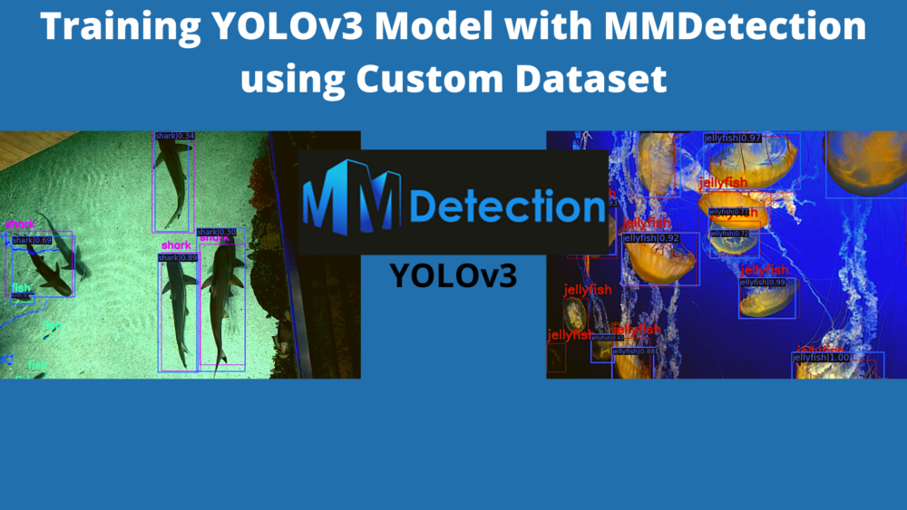
MMDetection toolbox offers a lot of pretrained models. In fact, as of writing this, we can find nearly 500 pretrained weights in the MMDetection repository. This number is so high because there are trained weights for every object detection architecture using different backbones and parameters. Along with many other models, it also offers trained weights for many variants of the YOLOv3 model. It will be pretty nice to check out how such a fast object detection model with PyTorch support works out on a custom dataset when fine-tuned using a pretrained checkpoint. It will also offer us some knowledge on how to use MMDetection’s YOLO models for custom dataset training. For that reason, we will be training a YOLOv3 model with MMDetection using a custom dataset in this tutorial.

If you want to learn about MMDetection more, please take a look at all the MMDetection posts here.

Also, if you want to get started with MMDetection training along with setting it up locally with CUDA (GPU) support, please take a look at the following posts:

• Install MMDetection on Ubuntu and Windows for RTX and GTX GPUs
• Image and Video Inference using MMDetection
• Getting Started with MMDetection Training for Object Detection
• Custom Dataset Training using MMDetection – Training using YOLOX

Topics to Cover in This Post

Now, let’s take a look at the topics that we will cover here in this post.

• We will first download the dataset. In this post, we will use the Aquarium Dataset from Roboflow. We will discuss the dataset in its own section.
• In the coding section, we will cover the following things:
  • First, we will prepare the dataset in the required Pascal VOC directory structure.
  • Second, we will briefly go over the PyTorch dataset preparation code. We will keep this section brief.
  • Then we will cover the configuration file to set up the dataset paths, training, and model configuration.
  • Next, we will carry out the training of the YOLOv3 model with MMDetection.
  • After training, we will use the trained model for running inference on images and videos.

Note: This post focuses mostly on how to convert and prepare custom datasets for MMDetection training and the training results. We will dive into the details of the code only in the very necessary parts. Other than that, all the code will be downloadable from the download section. If you wish to know in detail about all the code used in this post, please follow the series of tutorials mentioned in the above section.

Let’s get into the details of the post now.

The Aquarium Dataset

In this post, we will use the Aquarium dataset from Roboflow for training the YOLOv3 model using MMDetection. The dataset contains 638 images in total. This dataset contains images from two aquariums in the United States. The dataset provides annotations for different types of creatures in those aquariums. The classes for which annotations are available are fish, jellyfish, penguins, sharks, puffins, stingrays, and starfish. Following is an image showing the distributions of annotations instances from each class.

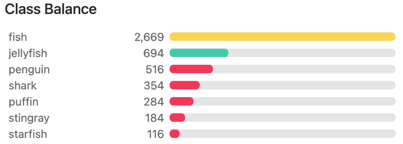
We can see that the puffin, stingray, and starfish classes are clearly underrepresented. This somewhat simulates a real-world scenario where we always don’t get perfect class distribution to train a model. This is a good dataset to check how the model performs.

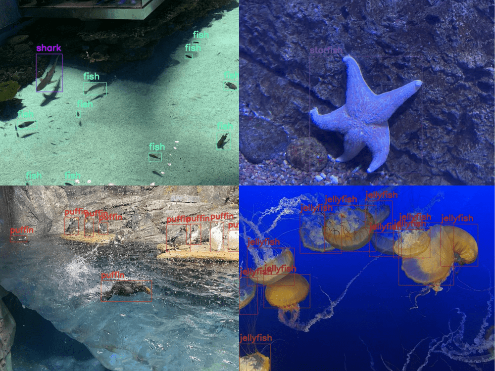
The above figure shows a few images from the dataset along with the annotations on the objects. You may take a look at the dataset in the directory before we start the training of the YOLOv3 model with MMDetection.

Downloading the Dataset

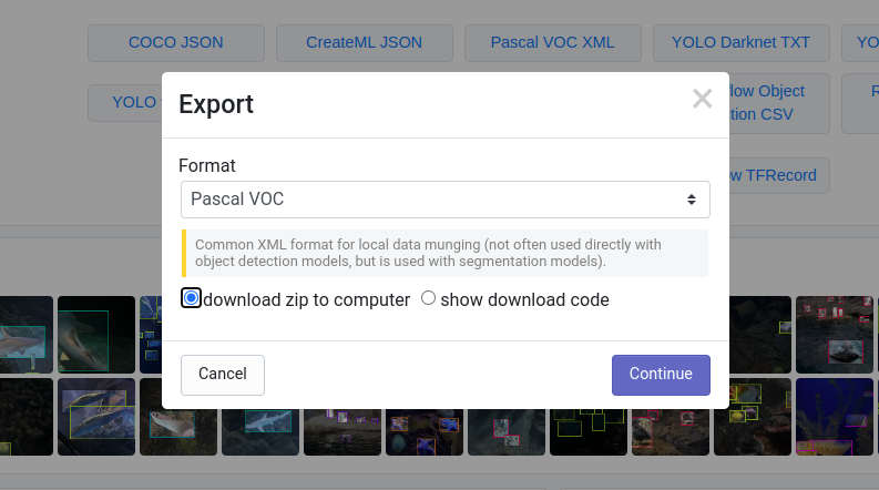
The dataset which we will use has already been split into 448 training, 127 validation, and 63 test images. So, we just need to download the dataset in the format that we need. We will need the dataset in the Pascal VOC XML format for later processing and bringing it to the correct directory structure. For now, you can download the zip file by clicking on the following link:

Download the Pascal VOC XML format of the dataset (you may need to sign in/sign up to download the dataset).

You will find the following directory structure after extracting the dataset:

Aquarium Combined.v2-raw-1024.voc
├── test
├── train
├── valid
├── README.dataset.txt
└── README.roboflow.txt

The train, valid, and test folders contain the JPEG images and corresponding XML files. We will use the training and validation sets for the training and validation loops. And we will use the test dataset for the final inference using the trained model.

In the next section, we will check out the directory structure of the entire project and where to keep this dataset.

Directory Structure

The following is the directory structure for the entire codebase in this tutorial.

├── checkpoints
│   └── yolov3_d53_320_273e_coco-421362b6.pth
├── input
│   ├── Aquarium Combined.v2-raw-1024.voc
│   ├── data_root
|   |   └── dataset
|   |       ├── Annotations
|   |       ├── ImageSets
|   |       └── JPEGImages
|   |
│   ├── inference_data
├── mmdetection
│   ├── configs
│   ...
│   └── setup.py
├── outputs
│   ├── inference_outputs
│   └── yolov3_d53_320_273e_coco
├── cfg.py
├── dataset.py
├── download_weights.py
├── inference_image.py
├── inference_video.py
├── prepare_voc_format.py
├── train.py
├── utils.py
└── weights.txt

• The checkpoints directory contains the pretrained checkpoint that we will use for fine-tuning.
• The input directory contains all the datasets that we need. We have already seen the contents of Aquarium Combined.v2-raw-1024.voc in the previous section. The data_root contains images and XML files from the original dataset’s training and validation set in the Pascal VOC directory structure which is essential for the custom training that we will carry out here. We will check out the code later for how to create this directory structure. And the inference_data directory contains test data from the original Aquarium dataset and a couple of videos for inferencing later on.
• We will clone the MMDetection repository to get access to the model and dataset configuration files. It is the mmdetection directory in the above block.
• The outputs directory contains both, the training as well as the inference outputs.
• Directly inside the parent project directory, there are Python code files which we will check out in the coding section. The weights.txt file contains the URLs of all the pretrained downloadable weights from MMDetection. This file is generated by executing the download_weights.py file.

You will get access to the inference data and all the Python code files when downloading the zip file for this post.

Training YOLOv3 Model with MMDetection using Custom Dataset

Let’s get down to the practical aspects of the post without any further delay. We will carry out the following steps in the coding section:

• Clone the MMDetection repository.
• Download the YOLOv3 weights that we wish to fine-tune.
• Convert the JPEG and XML files to the Pascal VOC directory structure.
• Check out the code for preparing the PyTorch datasets and data loaders.
• Prepare the model, dataset, and training configuration file.
• Carry out the training.
• Use the trained model for running inference on images and videos.

Clone the MMDetection Library

We first need to clone the MMDetection toolbox/repository/library. Execute the following command directly inside the parent project directory.

Download Code

git clone https://github.com/open-mmlab/mmdetection.git

After cloning, you should see the mmdetection folder in the directory.

Download the Required Pretrained YOLOv3 Weights

In this post, we will use the yolov3_d53_320_273e_coco pretrained weights. So, what exactly is this model? We can find all the details about this dataset here. These are a few details about the dataset:

• It is a YOLOv3 model with the Darknet-53 backbone.
• It has been pretrained on the COCO dataset for 273 epochs and the final box AP was 27.9.

This mAP may not be very high. But this is a considerably fast object detection model and should give us real-time FPS even on moderate hardware.

The download_weights.py file contains the code to download any pretrained model that we want. We just need to provide the correct --weights flag for that model. We will not go into the details of the code here. If you are interested, you may have a look at the series posts mentioned in the introduction section which contains all the details of the code.

For now, let’s download the weights. Execute the following command from your command line/terminal.

python download_weights.py --weights yolov3_d53_320_273e_coco 

The output should be similar to the following.

python download_weights.py --weights yolov3_d53_320_273e_coco
Founds weights: https://download.openmmlab.com/mmdetection/v2.0/yolo/yolov3_d53_320_273e_coco/yolov3_d53_320_273e_coco-421362b6.pth

Downloading yolov3_d53_320_273e_coco-421362b6.pth
100%|███████████████████████████████████████| 248M/248M [00:22<00:00, 11.0MiB/s]

You will find the weights in the checkpoints directory.

Converting the Dataset To Pascal VOC Directory Structure

Now, it’s time to convert the original Aquarium dataset into the Pascal VOC directory structure. This is important because we will use an already existing dataset and data loader preparation code from MMDetection. This expects the directory format to be in the Pascal VOC directory structure.

The code for preparing this directory structure will go into the prepare_voc_format.py file.

The following code block contains all the import statements and the directory paths we need to deal with.

import os
import shutil
import cv2
import glob as glob

ROOT_DATA = os.path.join('input', 'data_root')
ROOT_IMAGE_PREFIX = os.path.join(ROOT_DATA, 'dataset')
ANNOT_FOLDER = os.path.join(ROOT_IMAGE_PREFIX, 'Annotations')
TEXT_FILE_IMAGE_SETS = os.path.join(ROOT_IMAGE_PREFIX, 'ImageSets', 'Main')
IMAGE_FOLDER = os.path.join(ROOT_IMAGE_PREFIX, 'JPEGImages')

os.makedirs(ROOT_DATA, exist_ok=True)
os.makedirs(ROOT_IMAGE_PREFIX, exist_ok=True)
os.makedirs(ANNOT_FOLDER, exist_ok=True)
os.makedirs(TEXT_FILE_IMAGE_SETS, exist_ok=True)
os.makedirs(IMAGE_FOLDER, exist_ok=True)

TRAIN_IMAGES_PATH = os.path.join(
    'input', 
    'Aquarium Combined.v2-raw-1024.voc', 
    'train'
)
TRAIN_XML_PATH = os.path.join(
    'input', 
    'Aquarium Combined.v2-raw-1024.voc', 
    'train'
)
VALID_IMAGES_PATH = os.path.join(
    'input', 
    'Aquarium Combined.v2-raw-1024.voc', 
    'valid'
)
VALID_XML_PATH = os.path.join(
    'input', 
    'Aquarium Combined.v2-raw-1024.voc', 
    'valid'
)

Apart from cv2, which we will use for reading the writing images, all other imports deal with directory paths.

From lines 6 to 10, we define the new Pascal VOC directory and subdirectory paths that we need. Then we create all of them from lines 12 to 16. This will create the exact structure as the original Pascal VOC data. The Annotations directory will contain all the XML files. The JPEGImages directory will contain the images. And ImageSets/Main will contain the text files with the names of the files to be used for training and validation.

From lines 18 to 37 we define the image and XML file paths of the original Aquarium dataset that we want to deal with.

The next code block contains three functions to create the text files, copy the XML annotations into the Annotations directory, and copy the images to the JPEGImages directory.

# Give split as 'train' or 'val', or 'test'.
def create_text_file_sets(orig_image_folder, save_folder, split='train'):
    all_images = glob.glob(os.path.join(orig_image_folder, '*.jpg'))
    with open(os.path.join(save_folder, split+'.txt'), 'w') as f:
        for i, image_name in enumerate(all_images):
            file_name = image_name.split('.jpg')[0].split(os.path.sep)[-1]
            f.writelines(file_name+'\n')

# Copy the XML files to `Annotations` folder.
def xml_to_annotations_folder(
    orig_xml_train_folder, orig_xml_valid_folder, save_folder
):
    train_xmls = glob.glob(os.path.join(orig_xml_train_folder, '*.xml'))
    for train_xml in train_xmls:
        file_name = train_xml.split('.xml')[0].split(os.path.sep)[-1]
        shutil.copy(
            train_xml,
            os.path.join(save_folder, file_name+'.xml')
        )

    valid_xmls = glob.glob(os.path.join(orig_xml_valid_folder, '*.xml'))
    for valid_xml in valid_xmls:
        file_name = valid_xml.split('.xml')[0].split(os.path.sep)[-1]
        shutil.copy(
            valid_xml,
            os.path.join(save_folder, file_name+'.xml')
        )

# Copy the images to the `JPEGImages` folder.
def images_to_jpegimages_folder(
    orig_image_train_folder, orig_image_valid_folder, save_folder
):
    train_images = glob.glob(os.path.join(orig_image_train_folder, '*.jpg'))
    for train_image in train_images:
        file_name = train_image.split('.jpg')[0].split(os.path.sep)[-1]
        image = cv2.imread(os.path.join(train_image))
        cv2.imwrite(os.path.join(save_folder, file_name+'.jpg'), image)

    valid_images = glob.glob(os.path.join(orig_image_valid_folder, '*.jpg'))
    for valid_image in valid_images:
        file_name = valid_image.split('.jpg')[0].split(os.path.sep)[-1]
        image = cv2.imread(os.path.join(valid_image))
        cv2.imwrite(os.path.join(save_folder, file_name+'.jpg'), image)

The create_text_file_sets function creates the train and val text files. The xml_to_annotations_folder functions copies all the original XML files into data_root/dataset/Annotations. And images_to_jpegimages_folder function copies all the images to data_root/dataset/JPEGImages.

Now, we just need to execute the functions while providing the correct arguments.

# Create train image set text file.
create_text_file_sets(TRAIN_IMAGES_PATH, TEXT_FILE_IMAGE_SETS, 'train')

# Create validation image set text file.
create_text_file_sets(VALID_IMAGES_PATH, TEXT_FILE_IMAGE_SETS, 'val')

# Create XML files in annotations folder.
xml_to_annotations_folder(
    TRAIN_XML_PATH, VALID_XML_PATH, save_folder=ANNOT_FOLDER
)

# Create JPEG images in JPEGImages folder.
images_to_jpegimages_folder(
    TRAIN_IMAGES_PATH, VALID_IMAGES_PATH, IMAGE_FOLDER
)

Executing the following command will create the required structure for us.

python prepare_voc_format.py

We can find the data in the input directory now.

Dataset and Data Loader Preparation Code

Now, it’s time to check out the code that will prepare the PyTorch datasets and data loaders for us. This is actually a custom dataset code that is already in the MMDetection documentation here.

In all fairness, we will use almost the entirety of the code as it is, except for a small change. We need to provide the class names right after defining the XMLCustomDataset class and before the __init__ method begins.

The code for this is present in the dataset.py file. Although, we will not go into the details of the code here as almost all of it is self-explanatory, let’s just check out what the first part of the code along with our custom classes looks like.

@DATASETS.register_module()
class XMLCustomDataset(CustomDataset):
    """XML dataset for detection.

    Args:
        min_size (int | float, optional): The minimum size of bounding
            boxes in the images. If the size of a bounding box is less than
            ``min_size``, it would be add to ignored field.
        img_subdir (str): Subdir where images are stored. Default: JPEGImages.
        ann_subdir (str): Subdir where annotations are. Default: Annotations.
    """
    CLASSES = (
        'fish', 'jellyfish', 'penguin',
        'shark', 'puffin', 'stingray',
        'starfish'
        )
    def __init__(self,
                 min_size=None,
                 img_subdir='JPEGImages',
                 ann_subdir='Annotations',
                 **kwargs):

        assert self.CLASSES or kwargs.get(
            'classes', None), 'CLASSES in `XMLDataset` can not be None.'
        self.img_subdir = img_subdir
        self.ann_subdir = ann_subdir
        super(XMLCustomDataset, self).__init__(**kwargs)
        self.cat2label = {cat: i for i, cat in enumerate(self.CLASSES)}
        self.min_size = min_size
        print(self.CLASSES)

We have the CLASSES tuple right after defining the XMLCustomDataset class which contains all the class names from our dataset.

The rest of the class contains the methods for reading the annotations files, reading the images, and preparing the ground truth labels. Please go through the code once if you wish to know about these methods in detail.

Setting Up the Configuration File

The next important part is setting up the configuration file properly. It will contain the following things:

• Proper paths to the training and validation set.
• The correct number of classes in the dataset.
• The desired configurations for the model.
• The learning parameters/hyperparameters.

The configuration file details will go into the cfg.py file.

The following block contains all the code for the configuration file, but we will discuss the important parts only.

Starting with the import statements, loading the default configuration file and paths to the datasets.

from mmcv import Config
from mmdet.apis import set_random_seed
from dataset import XMLCustomDataset

cfg = Config.fromfile('mmdetection/configs/yolo/yolov3_d53_320_273e_coco.py')
print(f"Default Config:\n{cfg.pretty_text}")

# Modify dataset type and path.
cfg.dataset_type = 'XMLCustomDataset'
cfg.data_root = 'input/data_root/'

cfg.data.test.type = 'XMLCustomDataset'
cfg.data.test.data_root = 'input/data_root/'
cfg.data.test.ann_file = 'dataset/ImageSets/Main/val.txt'
cfg.data.test.img_prefix = 'dataset/'

cfg.data.train.type = 'XMLCustomDataset'
cfg.data.train.data_root = 'input/data_root/'
cfg.data.train.ann_file = 'dataset/ImageSets/Main/train.txt'
cfg.data.train.img_prefix = 'dataset/'

cfg.data.val.type = 'XMLCustomDataset'
cfg.data.val.data_root = 'input/data_root/'
cfg.data.val.ann_file = 'dataset/ImageSets/Main/val.txt'
cfg.data.val.img_prefix = 'dataset/' 

Next are the model and training-related parameters.

# Batch size (samples per GPU).
cfg.data.samples_per_gpu = 16

# Modify number of classes as per the model head.
cfg.model.bbox_head.num_classes = 7
# Comment/Uncomment this to training from scratch/fine-tune according to the 
# model checkpoint path. 
cfg.load_from = 'checkpoints/yolov3_d53_320_273e_coco-421362b6.pth'

# The original learning rate (LR) is set for 8-GPU training.
# We divide it by 8 since we only use one GPU.
cfg.optimizer.lr = 0.008 / 8
cfg.lr_config.warmup = None
cfg.log_config.interval = 5

This code uses a batch size of 16. If you run into memory limitations (OOM errors), then please reduce the batch size. Other than that, we configure the number of classes for the YOLO detection head and also the pretrained checkpoint path.

The learning rate is 0.001 and we are not using any warmup here.

The rest of the configurations deal with the output directory and logging of the results.

# The output directory for training. As per the model name.
cfg.work_dir = 'outputs/yolov3_d53_320_273e_coco'
# Evaluation Metric.
cfg.evaluation.metric = 'mAP'
# Evaluation times.
cfg.evaluation.interval = 1
# Checkpoint storage interval.
cfg.checkpoint_config.interval = 15

# Set random seed for reproducible results.
cfg.seed = 0
set_random_seed(0, deterministic=False)
cfg.gpu_ids = range(1)
cfg.device = 'cuda'
cfg.runner.max_epochs = 100

# We can also use tensorboard to log the training process
cfg.log_config.hooks = [
    dict(type='TextLoggerHook'),
    dict(type='TensorboardLoggerHook')]

# We can initialize the logger for training and have a look
# at the final config used for training
print('#'*50)
print(f'Config:\n{cfg.pretty_text}')

We will be saving the checkpoints every 15 epochs and our evaluation metric is mAP. As the evaluation interval is 1, the evaluation will be carried on the validation set after each epoch showing the AP for each class and the mAP as well.

Training the YOLOv3 Model on the Aquarium Dataset using MMDetection

Now it is time to train the model. The training script is quite simple. The train.py file contains all the code to start the training.

from mmdet.datasets import build_dataset
from mmdet.models import build_detector
from mmdet.apis import train_detector
from cfg import cfg

import os.path as osp
import mmcv

# Build dataset
datasets = [build_dataset(cfg.data.train)]

# Build the detector
model = build_detector(cfg.model)
# Add an attribute for visualization convenience
model.CLASSES = datasets[0].CLASSES

# Create work_dir
mmcv.mkdir_or_exist(osp.abspath(cfg.work_dir))
train_detector(model, datasets, cfg, distributed=False, validate=True)

We just prepare the datasets, load the configuration file, initialize the model, and start the training.

Note that the training shown in this post has been done on a machine with 10GB RTX 3080 GPU, 10th generation i7 CPU, and 32 GB RAM. Your training time may vary according to the hardware used.

To start the training, execute the following command from the parent project directory.

python train.py

The following block shows the mAP from the final epoch evaluation.

+-----------+-----+------+--------+-------+
| class     | gts | dets | recall | ap    |
+-----------+-----+------+--------+-------+
| fish      | 459 | 1189 | 0.826  | 0.652 |
| jellyfish | 155 | 254  | 0.884  | 0.849 |
| penguin   | 104 | 279  | 0.817  | 0.594 |
| shark     | 57  | 334  | 0.825  | 0.600 |
| puffin    | 74  | 165  | 0.635  | 0.482 |
| stingray  | 33  | 196  | 0.818  | 0.694 |
| starfish  | 27  | 61   | 0.741  | 0.686 |
+-----------+-----+------+--------+-------+
| mAP       |     |      |        | 0.651 |
+-----------+-----+------+--------+-------+
2022-06-25 22:40:51,374 - mmdet - INFO - Epoch(val) [100][127]	AP50: 0.6510, mAP: 0.6511

We have an mAP of more than 65%. Not bad considering we used a small resolution during training (320×320) and we did not have that many training images as well.

The following are the TensorBoard logs that are saved to the disk.

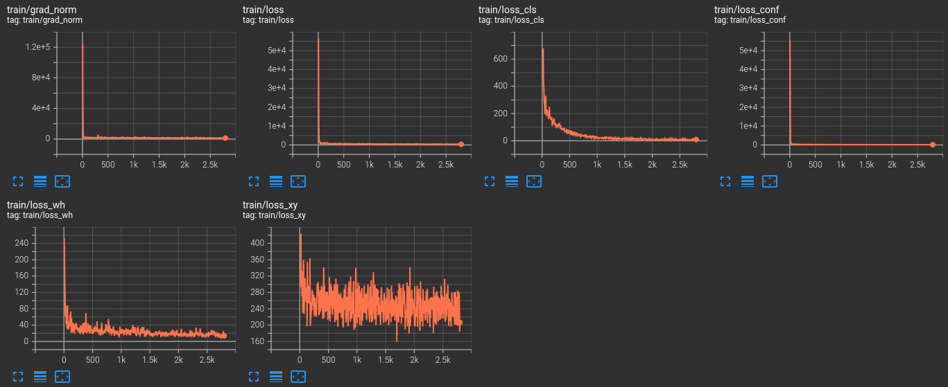
You can also view the logs on your own using the following command from the terminal from the outputs/yolov3_d53_320_273e_coco/tf_logs directory.

tensorboard --logdir ./

Next, go to the http://localhost:6006/ URL to see the logs.

Inference using the Trained Model

Right now, we have the trained YOLOv3 model in the outputs/yolov3_d53_320_273e_coco directory. We will use the model saved after the final epoch for image and video inference.

Inference on Images

For running inference on images we will use the test images from the Aquarium dataset. Although the test set comes with the original dataset, you will also find it in input/inference_data/test_images if you have downloaded the zip file for this post. This folder contains both the images and the XML files as well. So, while running inference on these images, we will also annotate the objects with the ground truth bounding boxes along with the predictions. This will give us a good idea of how many objects the trained YOLOv3 model detects correctly.

The code for this is present in the inference_image.py file. It is a straightforward code and we will not cover the code here. Be sure to check it out once on your own.

Execute the image inference script using the following command.

python inference_image.py --weights outputs/yolov3_d53_320_273e_coco/epoch_100.pth --threshold 0.25

We are setting a detection threshold of 25% here.

Let’s check out a few predictions here.

• 

• 

• 

• 

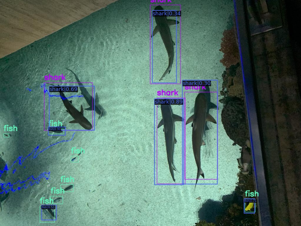
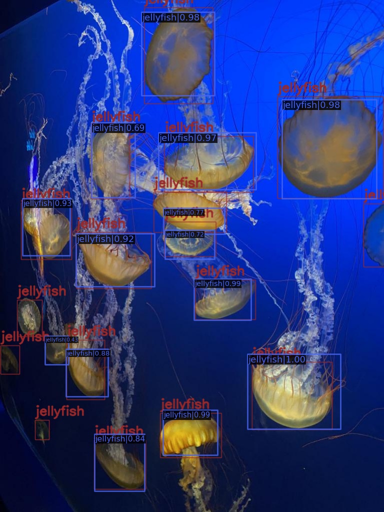
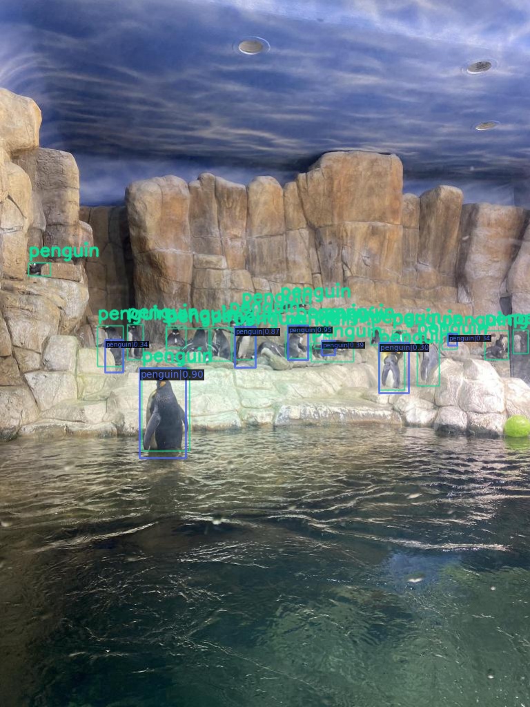
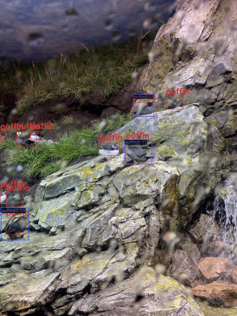
The colored annotations in the images are the ground truths and the blue text on the black background shows the prediction results. We can clearly see the limitations here. The model is not performing well on crowded images and smaller objects like fish. The puffin class was underrepresented and therefore the model is not performing well here.

Inference on Videos

We will carry out inference on two videos here. The code for this is present in the inference_video.py file.

Note that the inference shown in this post has been done on a machine with 10GB RTX 3080 GPU, 10th generation i7 CPU, and 32 GB RAM. Your FPS may vary according to the hardware used.

Let’s run the inference on the first video.

python inference_video.py --weights outputs/yolov3_d53_320_273e_coco/epoch_100.pth --input input/inference_data/video_1.mp4 --threshold 0.25

On the RTX 3080 GPU, it ran with around 85 FPS.

We can see that the model is performing well on the shark and fish classes, but not so well on the stingray class. In fact, it is predicting some of the stingrays as fish.

Let’s check out another inference, where we have only the stingray class.

python inference_video.py --weights outputs/yolov3_d53_320_273e_coco/epoch_100.pth --input input/inference_data/video_2.mp4 --threshold 0.25

The model is clearly facing difficulty here as well. We can attribute this to the less number of instances present for this class in the dataset and how important it can be to deal with such issues.

Summary and Conclusion

In this post, we learned how to carry out training of a YOLOv3 model with MMDetection using a custom dataset. We used the Aquarium dataset for this. The inference results also showed us how class imbalance can negatively affect a model’s performance. I hope that you learned something new from this post.

If you have any doubts, thoughts, or suggestions, please leave them in the comment section. I will surely address them.

You can contact me using the Contact section. You can also find me on LinkedIn, and Twitter.