Custom Dataset Training using MMDetection

Writing our own object detection training pipelines can be difficult. Even more so when trying to implement the loss functions and metrics from scratch. Rather we can use tools like MMDetection which do the heavy-lifting for us. And we can completely focus on preparing a good dataset, choosing the right model, and carrying out a lot of experiments. So, in this tutorial, we will be training an MMDetection model on a custom dataset.

For the past few posts, we have been covering a lot of topics in MMDetection. We started with the installation of MMCV and MMDetection. Then after the simple inference using some pretrained models, we carried out training on the Pascal VOC 2007 dataset. That did not require any custom data preparation or dataset class. Now, it’s time that we do a custom dataset training with YOLOx and MMDetection on the GTSDB dataset.

This is the fourth post in the Getting Started with MMDetection for Object Detection series.

• Install MMDetection on Ubuntu and Windows for RTX and GTX GPUs.
• Image and Video Inference using MMDetection.
• Getting Started with MMDetection Training for Object Detection.
• Custom Dataset Training using MMDetection

Now, let’s take a look at what we will cover in this tutorial:

• We will start by exploring the dataset. We will use the German Traffic Sign Detection Benchmark dataset in this tutorial. This section will also cover how we structure the dataset.
• Then will have an overview of the steps that we will follow to carry out the custom dataset training using the MMDetection.
• Next, we will move on to the coding section of the tutorial.
• After training the model, we will also carry out inference on a video containing different traffic signs.

The German Traffic Sign Detection Benchmark Dataset

It is popularly known as the GTSDB dataset as well. It contains a total of 900 images. Out of these, 600 images are labeled and we will divide them into a training and a validation set. We will use these two sets for the training phase of the model.

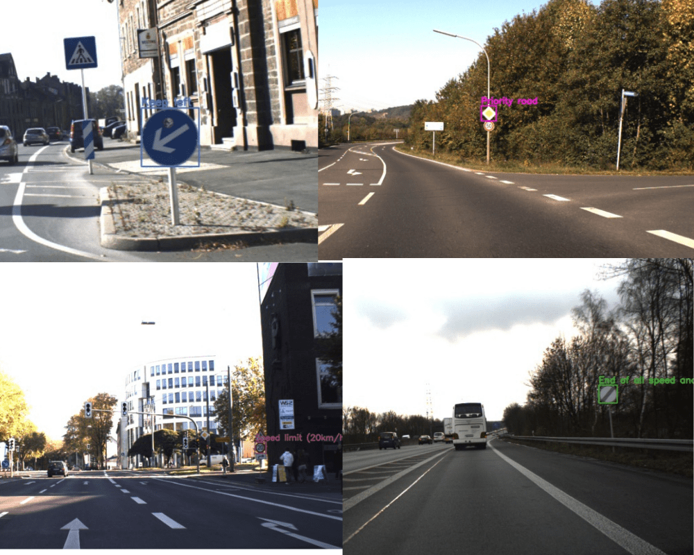
Out of the test images, we will use a few of them for inference after we train the model.

The dataset contains 43 classes and a few of them are:

• ‘Speed limit (120km/h)’, ‘No passing’, ‘No passing for vehicles over 3.5 metric tons’.

Although you can find the original dataset here, we need the dataset in the Pascal VOC directory structure for the custom training using MMDetection. So, you will need to first download the prepared dataset from Kaggle.

The Custom Dataset Structure

For this custom training using MMDetection, we will use the dataset in the Pascal VOC structure.

After you download and extract the dataset, you will find the input directory in the following structure.

.
├── data_root
│   └── dataset
│       ├── Annotations
│       │   ├── 00000.xml
│       │   ├── 00001.xml
│       │   ...
│       │   └── 00599.xml
│       ├── ImageSets
│       │   └── Main
│       │       ├── train.txt
│       │       └── val.txt
│       └── JPEGImages
│           ├── 00000.jpg
│           ├── 00001.jpg
│           ...
│           └── 00599.jpg
├── inference_data
│   ├── 00080.ppm
│   ├── 00082.ppm
│   ├── 00265.ppm
│   └── video_1.mp4
├── classes_list.txt

7 directories, 1018 files

So, inside the input directory, we have the data_root/dataset subdirectory structure.

• The Annotations folder contains all the XML files containing the ground truth bounding box and class label data.
• The JPEGImages folder contains all the images in .jpg format. The original images were available in .ppm format. But we convert the images to .jpg format to easily work with them.
• The inference_data folder contains a few images from the test set and a video that we will use for inference.
• Finally, the classes_list.txt file contains all the class names from the dataset in a list format.

In the next section, we will see where to keep the input data directory for the project.

The Project Directory Structure

The following is the directory structure for the entire project.

├── checkpoints
│   └── yolox_l_8x8_300e_coco_20211126_140236-d3bd2b23.pth
├── input
│   ├── data_root
│   │   └── dataset
│   ├── inference_data
│   │   ├── 00080.ppm
│   │   ├── 00082.ppm
│   │   ├── 00265.ppm
│   │   └── video_1.mp4
│   └── classes_list.txt
├── mmdetection
│   ├── configs
│   │   ├── albu_example
│   ...
│   └── setup.py
├── outputs
│   ├── yolox_l_8x8_300e_coco
│   │   ├── tf_logs
│   │   ├── best_mAP_epoch_55.pth
│   │   ...
│   │   └── None.log.json
│   └── video_1.mp4
├── cfg.py
├── dataset.py
├── download_weights.py
├── inference_image.py
├── inference_video.py
├── train.py
└── weights.txt

134 directories, 73 files

We have already seen the structure of the input directory. Let’s go through the other parts here.

• The checkpoints directory contains the pretrained model checkpoint that we will use for fine-tuning. We will discuss the model that we will use briefly in one of the further sections.
• We will also need to clone the MMDetection repository, that is the mmdetection directory in the above block.
• The outputs directory will contain all the outputs from training and inference.
• We have five Python files in total that we will discuss in the coding section.
• The weights.txt file contains a list of almost all the pretrained model URLs from the MMDetection toolbox.

You will get access to all the code files when downloading the zip file for this tutorial.

Steps for Custom Dataset Training using MMDetection

First, let’s list out all the steps that we will cover for this custom object detection training using MMDetection.

• We will start with cloning the MMDetection repository. We will need access to the repository’s the configuration files.
• Then we will download the pretrained weights which we will use for fine-tuning. We will use one of the YOLOX models. Specifically, we will use the YOLOX-l model. We will not go through the details of the YOLOX model in this tutorial. Rather we will focus entirely on the custom training part. We are using this model as this gave appropriately good results while being reasonably fast to train.
• Next, we will check out the custom dataset preparation script which will read the images and labels from the VOC-like dataset directory.
• Then we will prepare the configuration file for training. This contains the model as well as dataset configuration.
• The next step is to carry out the training.
• After the training, we will run inference on a few images and a video to check the performance of our trained model.

Note that some of the coding parts are going to be similar to the previous tutorial. We will not go into the details of these parts and rather focus our attention on the most important parts in the custom object detection training pipeline.

Training on Custom Dataset using MMDetection and YOLOX

Let’s get into the coding section now. We will follow each step as mentioned in the previous section.

Clone the MMDetection Repository

We will first need to clone the MMDetection repository. For setting the model and dataset configuration properly, we will need to access the mmdetection/configs directory. For that, we need to clone the repository first.

Download Code

In the parent project directory, execute the following command to clone the repository.

git clone https://github.com/open-mmlab/mmdetection.git

You should be able to see the mmdetection directory after the process completes.

Downloading the YOLOX Pretrained Weights

The code for downloading the pretrained weights is present in the download_weights.py script. The code for this remains exactly the same as we had in the previous tutorial. So, we will not cover that in detail here again. The following block contains the entire code for download_weights.py.

import os
import requests
import yaml
import glob as glob
import argparse

from tqdm import tqdm

def download_weights(url, file_save_name):
    """
    Download weights for any model.

    :param url: Download URL for the weihgt file.
    :param file_save_name: String name to save the file on to disk.
    """
    data_dir = 'checkpoints'
    if not os.path.exists(data_dir):
        os.makedirs(data_dir)
    # Download the file if not present.
    if not os.path.exists(os.path.join(data_dir, file_save_name)):
        print(f"Downloading {file_save_name}")
        file = requests.get(url, stream=True)
        total_size = int(file.headers.get('content-length', 0))
        block_size = 1024
        progress_bar = tqdm(
            total=total_size, 
            unit='iB', 
            unit_scale=True
        )
        with open(os.path.join(data_dir, file_save_name), 'wb') as f:
            for data in file.iter_content(block_size):
                progress_bar.update(len(data))
                f.write(data)
        progress_bar.close()
    else:
        print('File already present')

def parse_meta_file():
    """
    Function to parse all the model meta files inside `mmdetection/configs`
    and return the download URLs for all available models.

    Returns:
        weights_list: List containing URLs for all the downloadable models.
    """
    root_meta_file_path = 'mmdetection/configs'
    all_metal_file_paths = glob.glob(os.path.join(root_meta_file_path, '*', 'metafile.yml'), recursive=True)
    weights_list = []
    for meta_file_path in all_metal_file_paths:
        with open(meta_file_path,'r') as f:
            yaml_file = yaml.safe_load(f)
            
        for i in range(len(yaml_file['Models'])):
            try:
                weights_list.append(yaml_file['Models'][i]['Weights'])
            except:
                for k, v in yaml_file['Models'][i]['Results'][0]['Metrics'].items():
                    if k == 'Weights':
                        weights_list.append(yaml_file['Models'][i]['Results'][0]['Metrics']['Weights'])
    return weights_list

def get_model(model_name):
    """
    Either downloads a model or loads one from local path if already 
    downloaded using the weight file name (`model_name`) provided.

    :param model_name: Name of the weight file. Most likely in the format
        retinanet_ghm_r50_fpn_1x_coco. SEE `weights.txt` to know weight file
        name formats and downloadable URL formats.

    Returns:
        model: The loaded detection model.
    """
    # Get the list containing all the weight file download URLs.
    weights_list = parse_meta_file()

    download_url = None
    for weights in weights_list:
        if model_name == weights.split('/')[-2]:
            print(f"Founds weights: {weights}\n")
            download_url = weights
            break

    assert download_url != None, f"{model_name} weight file not found!!!"

    # Download the checkpoint file.
    download_weights(
        url=download_url,
        file_save_name=download_url.split('/')[-1]
    )

def write_weights_txt_file():
    """
    Write all the model URLs to `weights.txt` to have a complete list and 
    choose one of them.
    EXECUTE `utils.py` if `weights.txt` not already present.
    `python utils.py` command will generate the latest `weights.txt` 
    file according to the cloned mmdetection repository.
    """
    # Get the list containing all the weight file download URLs.
    weights_list = parse_meta_file()
    with open('weights.txt', 'w') as f:
        for weights in weights_list:
            f.writelines(f"{weights}\n")
    f.close()

if __name__ == '__main__':
    write_weights_txt_file()
    
    parser = argparse.ArgumentParser()
    parser.add_argument(
    '-w', '--weights', default='yolox_l_8x8_300e_coco',
    help='weight file name'
    )
    args = vars(parser.parse_args())

    get_model(args['weights'])

If you are really interested in the code, please visit the previous tutorial which contains all the explanation for the above code.

The only thing that will change this time is that we will download the yolox_l_8x8_300e_coco pretrained weights. Execute the following command from your terminal/command line:

python download_weights.py --weights yolox_l_8x8_300e_coco

The output should be similar to the following:

Founds weights: https://download.openmmlab.com/mmdetection/v2.0/yolox/yolox_l_8x8_300e_coco/yolox_l_8x8_300e_coco_20211126_140236-d3bd2b23.pth

Downloading yolox_l_8x8_300e_coco_20211126_140236-d3bd2b23.pth
100%|████████████████████████████████████████217M/217M [00:20<00:00, 10.8MiB/s]

The weights will be downloaded into the checkpoints directory. The directory will be automatically created if not already present.

Custom Dataset Preparation for XML Type Dataset

Now it is time to prepare the custom XML style dataset. The code that we will use here has been adapted from the official MMDetection documentation. In fact, there is not much change in the code apart from adding a tuple containing all the class names in our dataset. We will add this tuple inside the custom dataset class just before the __init__ method.

The reason for so much less hassle is that we already have our dataset directory structure in the Pascal VOC format. So, the official code will take care of all the things and we just have to mention the new class names as per the dataset.

All the code here will go into the dataset.py file.

The following is the first code block containing the imports, the beginning the of class, and the __init__ method.

# Copyright (c) OpenMMLab. All rights reserved.
"""
Adapted from: https://mmdetection.readthedocs.io/en/latest/_modules/mmdet/datasets/xml_style.html
"""
import os.path as osp
import xml.etree.ElementTree as ET

import mmcv
import numpy as np
from PIL import Image

from mmdet.datasets.builder import DATASETS
from mmdet.datasets.custom import CustomDataset

@DATASETS.register_module()
class XMLCustomDataset(CustomDataset):
    """XML dataset for detection.

    Args:
        min_size (int | float, optional): The minimum size of bounding
            boxes in the images. If the size of a bounding box is less than
            ``min_size``, it would be add to ignored field.
        img_subdir (str): Subdir where images are stored. Default: JPEGImages.
        ann_subdir (str): Subdir where annotations are. Default: Annotations.
    """
    CLASSES = (
            'Speed limit (20km/h)', 'Speed limit (30km/h)', 'Speed limit (50km/h)', 
            'Speed limit (60km/h)', 'Speed limit (70km/h)', 'Speed limit (80km/h)', 
            'End of speed limit (80km/h)', 'Speed limit (100km/h)', 
            'Speed limit (120km/h)', 'No passing', 
            'No passing for vehicles over 3.5 metric tons', 
            'Right-of-way at the next intersection', 'Priority road', 'Yield', 
            'Stop', 'No vehicles', 'Vehicles over 3.5 metric tons prohibited', 
            'No entry', 'General caution', 'Dangerous curve to the left', 
            'Dangerous curve to the right', 'Double curve', 'Bumpy road', 
            'Slippery road', 'Road narrows on the right', 'Road work', 
            'Traffic signals', 'Pedestrians', 'Children crossing', 
            'Bicycles crossing', 'Beware of ice/snow', 'Wild animals crossing', 
            'End of all speed and passing limits', 'Turn right ahead', 
            'Turn left ahead', 'Ahead only', 'Go straight or right', 
            'Go straight or left', 'Keep right', 'Keep left', 'Roundabout mandatory', 
            'End of no passing', 'End of no passing by vehicles over 3.5 metric tons'
        )
    def __init__(self,
                 min_size=None,
                 img_subdir='JPEGImages',
                 ann_subdir='Annotations',
                 **kwargs):

        assert self.CLASSES or kwargs.get(
            'classes', None), 'CLASSES in `XMLDataset` can not be None.'
        self.img_subdir = img_subdir
        self.ann_subdir = ann_subdir
        super(XMLCustomDataset, self).__init__(**kwargs)
        self.cat2label = {cat: i for i, cat in enumerate(self.CLASSES)}
        self.min_size = min_size
        print(self.CLASSES)

There are a few important aspects to the above code block. The following points cover them.

• If we notice, we can see that we are importing the builder module as DATASETS. Internally, this is the module that prepares the datasets and the iterable data loaders among other tasks. And we register the XMLCustomDataset class with that module.
• The next important thing is the CLASSES tuple that we define right after the class and before the __init__() method. For the code to access the class names properly, it will have to be there only.
• In the parameters of the __init__ method, we can see that the parameters img_subdir and ann_subdir already have default values as JPEGImages and Annotations. This also confirms that using this class, we will need to have our dataset in the Pascal VOC directory structure which we already do.

The Rest of the Methods in the Custom Dataset Class

Now, let’s go briefly over the rest of the methods in the class. Note that all the following methods have one indentations block from the left as they are part of the XMLCustomDataset class. If you are downloading the code for this tutorial, you need not worry about this.

The following code block contains the method to load the annotations from the XML files.

def load_annotations(self, ann_file):
        """Load annotation from XML style ann_file.

        Args:
            ann_file (str): Path of XML file.

        Returns:
            list[dict]: Annotation info from XML file.
        """

        data_infos = []
        img_ids = mmcv.list_from_file(ann_file)
        for img_id in img_ids:
            filename = osp.join(self.img_subdir, f'{img_id}.jpg')
            xml_path = osp.join(self.img_prefix, self.ann_subdir,
                                f'{img_id}.xml')
            tree = ET.parse(xml_path)
            root = tree.getroot()
            size = root.find('size')
            if size is not None:
                width = int(size.find('width').text)
                height = int(size.find('height').text)
            else:
                img_path = osp.join(self.img_prefix, filename)
                img = Image.open(img_path)
                width, height = img.size
            data_infos.append(
                dict(id=img_id, filename=filename, width=width, height=height))

        return data_infos

The next method filters out all the images that are too small or do not have annotations in the XML files.

def _filter_imgs(self, min_size=32):
        """Filter images too small or without annotation."""
        valid_inds = []
        for i, img_info in enumerate(self.data_infos):
            if min(img_info['width'], img_info['height']) < min_size:
                continue
            if self.filter_empty_gt:
                img_id = img_info['id']
                xml_path = osp.join(self.img_prefix, self.ann_subdir,
                                    f'{img_id}.xml')
                tree = ET.parse(xml_path)
                root = tree.getroot()
                for obj in root.findall('object'):
                    name = str(obj.find('name').text)
                    if name in self.CLASSES:
                        valid_inds.append(i)
                        break
            else:
                valid_inds.append(i)
        return valid_inds

Now, the method to get the bounding box annotations and labels from the XML files.

def get_ann_info(self, idx):
        """Get annotation from XML file by index.

        Args:
            idx (int): Index of data.

        Returns:
            dict: Annotation info of specified index.
        """

        img_id = self.data_infos[idx]['id']
        xml_path = osp.join(self.img_prefix, self.ann_subdir, f'{img_id}.xml')
        tree = ET.parse(xml_path)
        root = tree.getroot()
        bboxes = []
        labels = []
        bboxes_ignore = []
        labels_ignore = []
        for obj in root.findall('object'):
            name = obj.find('name').text
            if name not in self.CLASSES:
                continue
            label = self.cat2label[name]
            difficult = obj.find('difficult')
            difficult = 0 if difficult is None else int(difficult.text)
            bnd_box = obj.find('bndbox')
            # TODO: check whether it is necessary to use int
            # Coordinates may be float type
            bbox = [
                int(float(bnd_box.find('xmin').text)),
                int(float(bnd_box.find('ymin').text)),
                int(float(bnd_box.find('xmax').text)),
                int(float(bnd_box.find('ymax').text))
            ]
            ignore = False
            if self.min_size:
                assert not self.test_mode
                w = bbox[2] - bbox[0]
                h = bbox[3] - bbox[1]
                if w < self.min_size or h < self.min_size:
                    ignore = True
            if difficult or ignore:
                bboxes_ignore.append(bbox)
                labels_ignore.append(label)
            else:
                bboxes.append(bbox)
                labels.append(label)
        if not bboxes:
            bboxes = np.zeros((0, 4))
            labels = np.zeros((0, ))
        else:
            bboxes = np.array(bboxes, ndmin=2) - 1
            labels = np.array(labels)
        if not bboxes_ignore:
            bboxes_ignore = np.zeros((0, 4))
            labels_ignore = np.zeros((0, ))
        else:
            bboxes_ignore = np.array(bboxes_ignore, ndmin=2) - 1
            labels_ignore = np.array(labels_ignore)
        ann = dict(
            bboxes=bboxes.astype(np.float32),
            labels=labels.astype(np.int64),
            bboxes_ignore=bboxes_ignore.astype(np.float32),
            labels_ignore=labels_ignore.astype(np.int64))
        return ann

And now, the final method to get the category IDs for the labels from the XML files.

def get_cat_ids(self, idx):
        """Get category ids in XML file by index.

        Args:
            idx (int): Index of data.

        Returns:
            list[int]: All categories in the image of specified index.
        """

        cat_ids = []
        img_id = self.data_infos[idx]['id']
        xml_path = osp.join(self.img_prefix, self.ann_subdir, f'{img_id}.xml')
        tree = ET.parse(xml_path)
        root = tree.getroot()
        for obj in root.findall('object'):
            name = obj.find('name').text
            if name not in self.CLASSES:
                continue
            label = self.cat2label[name]
            cat_ids.append(label)

        return cat_ids

These are all the methods of this class that we need. It is worthwhile to mention that we did not change any part of the code other than adding the class names.

The Configuration File

It is time to prepare the configuration file. It contains all the important details about the dataset and model that will be used by the training script for creating the data loaders and initializing the model.

The code for this will go into the cfg.py file.

The first code block here contains the import statements and loading of the default config file for the yolox_l_8x8_300e_coco model.

from mmcv import Config
from mmdet.apis import set_random_seed
from dataset import XMLCustomDataset

cfg = Config.fromfile('mmdetection/configs/yolox/yolox_l_8x8_300e_coco.py')
print(f"Default Config:\n{cfg.pretty_text}")

We are also importing the XMLCustomDataset here so that we can provide its name as the dataset type later on.

Configurations for the Dataset

The next part is quite important as we provide all the important configurations about the dataset here.

# Modify dataset type and path.
cfg.dataset_type = 'XMLCustomDataset'
cfg.data_root = 'input/data_root/'

cfg.data.test.type = 'XMLCustomDataset'
cfg.data.test.data_root = 'input/data_root/'
cfg.data.test.ann_file = 'dataset/ImageSets/Main/val.txt'
cfg.data.test.img_prefix = 'dataset/'

cfg.data.train.dataset.type = 'XMLCustomDataset'
cfg.data.train.dataset.data_root = 'input/data_root/'
cfg.data.train.dataset.ann_file = 'dataset/ImageSets/Main/train.txt'
cfg.data.train.dataset.img_prefix = 'dataset/'

cfg.data.val.type = 'XMLCustomDataset'
cfg.data.val.data_root = 'input/data_root/'
cfg.data.val.ann_file = 'dataset/ImageSets/Main/val.txt'
cfg.data.val.img_prefix = 'dataset/'

cfg.data.train.pipeline = [
    dict(type='Mosaic', img_scale=(640, 640), pad_val=114.0),
    dict(
        type='RandomAffine',
        scaling_ratio_range=(0.1, 2),
        border=(-320, -320)),
    dict(
        type='MixUp',
        img_scale=(640, 640),
        ratio_range=(0.8, 1.6),
        pad_val=114.0),
    dict(type='YOLOXHSVRandomAug'),
    dict(type='RandomFlip', flip_ratio=0.0),
    dict(type='Resize', img_scale=(640, 640), keep_ratio=True),
    dict(
        type='Pad',
        pad_to_square=True,
        pad_val=dict(img=(114.0, 114.0, 114.0))),
    dict(
        type='FilterAnnotations',
        min_gt_bbox_wh=(1, 1),
        keep_empty=False),
    dict(type='DefaultFormatBundle'),
    dict(type='Collect', keys=['img', 'gt_bboxes', 'gt_labels'])
    ]

# Batch size (samples per GPU).
cfg.data.samples_per_gpu = 2

We start with providing the dataset type which is the name of the custom dataset class and also the dataset root path.

Then we provide the dataset type, the data root path, text annotation file paths, and the image prefix file paths. We do this for the training, validation, and test set. But note that during the training procedure, the train data will be used for training and val data for validation. The test data will not be used. It will only be used if we specifically write a test script for it after the training completes so that we can test it on a test set. As we are not doing that here, so, we just provide the same paths as the val data for the test but it will be ignored during training.

One of the most important parts begins from line 25. Here we customize the cfg.data.train.pipeline that defines all the transforms and augmentations that are applied to the training dataset. We make a simple yet important modification here. Under normal circumstances, we do not need to modify this. But remember that we are using a traffic sign detection dataset that has the notion of left/right up/down in its signs. For that reason specifically, we cannot use the RandomFlip augmentation. So, we make the flip_ratio for this augmentation as 0 on line 37. We leave the rest of the transforms just as they are.

The final thing here is the samples_per_gpu configuration which is the batch size per GPU. The value here is 2, so at most 2 samples will be loaded per batch onto a GPU.

Configurations for the Model

The following block contains all the model-related configurations and a few training-related hyperparameter-based configurations.

# Modify number of classes as per the model head.
cfg.model.bbox_head.num_classes = 43
# Comment/Uncomment this to training from scratch/fine-tune according to the 
# model checkpoint path. 
cfg.load_from = 'checkpoints/yolox_l_8x8_300e_coco_20211126_140236-d3bd2b23.pth'

# The original learning rate (LR) is set for 8-GPU training.
# We divide it by 8 since we only use one GPU.
cfg.optimizer.lr = 0.0008 / 8
cfg.lr_config.warmup = None
cfg.log_config.interval = 5

As general in all of the YOLO models, YOLOX also has a bounding box head. So, we configure the model.bbox_head.num_classes to provide the proper number of classes in the dataset.

Note, that printing the default configuration file at the beginning helps to figure out all the configurations that we may need to modify for proper training.

Then we provide the path of the pretrained checkpoint that we want to load the weights from and fine-tune.

Next are the learning rate, the warmup for the learning rate which is None, and the log configuration interval. MMDetection always considers every configuration for multiple GPUs. So, when training on a single GPU, we divide the learning rate by 8. Here, the final learning rate is 0.0001. This is a bit lower than usual as we are fine-tuning from a pretrained checkpoint.

Rest of the Configurations

The following are the rest of the configurations that we need.

# The output directory for training. As per the model name.
cfg.work_dir = 'outputs/yolox_l_8x8_300e_coco'
# Evaluation Metric.
cfg.evaluation.metric = 'mAP'
cfg.evaluation.save_best = 'mAP'
# Evaluation times.
cfg.evaluation.interval = 1
# Checkpoint storage interval.
cfg.checkpoint_config.interval = 15

# Set random seed for reproducible results.
cfg.seed = 0
set_random_seed(0, deterministic=False)
cfg.gpu_ids = range(1)
cfg.device = 'cuda'
cfg.runner.max_epochs = 100

# We can also use tensorboard to log the training process
cfg.log_config.hooks = [
    dict(type='TextLoggerHook'),
    dict(type='TensorboardLoggerHook')]

# We can initialize the logger for training and have a look
# at the final config used for training
print('#'*50)
print(f'Config:\n{cfg.pretty_text}')

We configure the following things:

• The working directory to save the training outputs (models and logs).
• The evaluation metrics and also the configuration to save the best model as per the highest mAP metric.
• The evaluation interval. The code will evaluate through the validation dataset after every epoch as the value is 1 here.
• The checkpoint interval. Models will be saved to disk after every 15 epochs.
• It is quite important to mention that we want to use the 'cuda' device, or else the training may throw an error (line 78).
• We will be training for 100 epochs.
• TensoBoard will monitor all the metric and loss plots.

This is all we need for the configuration file.

The Training Script

The training script is the simplest of all and nothing changes compared to the previous tutorial.

The code for the training script will go into the train.py file.

from mmdet.datasets import build_dataset
from mmdet.models import build_detector
from mmdet.apis import train_detector
from cfg import cfg

import os.path as osp
import mmcv

# Build dataset
datasets = [build_dataset(cfg.data.train)]

# Build the detector
model = build_detector(cfg.model)
# Add an attribute for visualization convenience
model.CLASSES = datasets[0].CLASSES

# Create work_dir
mmcv.mkdir_or_exist(osp.abspath(cfg.work_dir))
train_detector(model, datasets, cfg, distributed=False, validate=True)

We build the dataset, and the model, create the working directory and start the training.

Execute train.py for Custom Dataset Training using MMDetection and YOLOX

Note: All the training, validation, and inference shown in this post have been done on a machine with 10 GB RTX 3080 GPU, i7 10th generation CPU, and 32 GB of RAM. Your training and inference speed may vary depending on the hardware.

Open the terminal/command line from the parent project directory and execute the following command.

python train.py 

The following are the best and last evaluation results from the training phase.

+----------------------------------------------------+-----+------+--------+-------+
| class                                              | gts | dets | recall | ap    |
+----------------------------------------------------+-----+------+--------+-------+
| Speed limit (20km/h)                               | 1   | 7    | 0.000  | 0.000 |
| Speed limit (30km/h)                               | 7   | 65   | 1.000  | 0.651 |
| Speed limit (50km/h)                               | 16  | 59   | 1.000  | 0.733 |
| Speed limit (60km/h)                               | 2   | 25   | 1.000  | 0.091 |
| Speed limit (70km/h)                               | 11  | 33   | 0.727  | 0.354 |
| Speed limit (80km/h)                               | 6   | 34   | 1.000  | 0.683 |
| End of speed limit (80km/h)                        | 0   | 2    | 0.000  | 0.000 |
| Speed limit (100km/h)                              | 9   | 20   | 0.778  | 0.661 |
| Speed limit (120km/h)                              | 5   | 14   | 0.800  | 0.362 |
| No passing                                         | 2   | 15   | 1.000  | 1.000 |
| No passing for vehicles over 3.5 metric tons       | 10  | 16   | 1.000  | 0.977 |
| Right-of-way at the next intersection              | 5   | 31   | 0.800  | 0.360 |
| Priority road                                      | 11  | 67   | 1.000  | 0.986 |
| Yield                                              | 9   | 27   | 1.000  | 0.967 |
| Stop                                               | 2   | 14   | 1.000  | 1.000 |
| No vehicles                                        | 2   | 3    | 0.500  | 0.500 |
| Vehicles over 3.5 metric tons prohibited           | 2   | 2    | 0.000  | 0.000 |
| No entry                                           | 7   | 12   | 1.000  | 1.000 |
| General caution                                    | 2   | 21   | 1.000  | 0.222 |
| Dangerous curve to the left                        | 0   | 5    | 0.000  | 0.000 |
| Dangerous curve to the right                       | 5   | 5    | 0.000  | 0.000 |
| Double curve                                       | 1   | 8    | 0.000  | 0.000 |
| Bumpy road                                         | 2   | 9    | 0.000  | 0.000 |
| Slippery road                                      | 2   | 16   | 0.000  | 0.000 |
| Road narrows on the right                          | 0   | 3    | 0.000  | 0.000 |
| Road work                                          | 6   | 35   | 0.667  | 0.237 |
| Traffic signals                                    | 3   | 19   | 0.000  | 0.000 |
| Pedestrians                                        | 1   | 2    | 0.000  | 0.000 |
| Children crossing                                  | 1   | 17   | 1.000  | 0.500 |
| Bicycles crossing                                  | 0   | 10   | 0.000  | 0.000 |
| Beware of ice/snow                                 | 6   | 14   | 1.000  | 0.737 |
| Wild animals crossing                              | 0   | 2    | 0.000  | 0.000 |
| End of all speed and passing limits                | 0   | 2    | 0.000  | 0.000 |
| Turn right ahead                                   | 1   | 4    | 0.000  | 0.000 |
| Turn left ahead                                    | 0   | 16   | 0.000  | 0.000 |
| Ahead only                                         | 1   | 15   | 1.000  | 1.000 |
| Go straight or right                               | 3   | 6    | 0.333  | 0.333 |
| Go straight or left                                | 0   | 1    | 0.000  | 0.000 |
| Keep right                                         | 5   | 41   | 1.000  | 1.000 |
| Keep left                                          | 0   | 5    | 0.000  | 0.000 |
| Roundabout mandatory                               | 2   | 6    | 1.000  | 1.000 |
| End of no passing                                  | 0   | 6    | 0.000  | 0.000 |
| End of no passing by vehicles over 3.5 metric tons | 4   | 4    | 0.500  | 0.417 |
+----------------------------------------------------+-----+------+--------+-------+
| mAP                                                |     |      |        | 0.478 |
+----------------------------------------------------+-----+------+--------+-------+
.
.
.
+----------------------------------------------------+-----+------+--------+-------+
| class                                              | gts | dets | recall | ap    |
+----------------------------------------------------+-----+------+--------+-------+
| Speed limit (20km/h)                               | 1   | 6    | 0.000  | 0.000 |
| Speed limit (30km/h)                               | 7   | 52   | 1.000  | 0.663 |
| Speed limit (50km/h)                               | 16  | 55   | 1.000  | 0.739 |
| Speed limit (60km/h)                               | 2   | 22   | 1.000  | 0.095 |
| Speed limit (70km/h)                               | 11  | 32   | 0.727  | 0.345 |
| Speed limit (80km/h)                               | 6   | 32   | 1.000  | 0.654 |
| End of speed limit (80km/h)                        | 0   | 2    | 0.000  | 0.000 |
| Speed limit (100km/h)                              | 9   | 19   | 0.778  | 0.664 |
| Speed limit (120km/h)                              | 5   | 14   | 0.800  | 0.362 |
| No passing                                         | 2   | 13   | 1.000  | 1.000 |
| No passing for vehicles over 3.5 metric tons       | 10  | 16   | 1.000  | 0.977 |
| Right-of-way at the next intersection              | 5   | 31   | 1.000  | 0.435 |
| Priority road                                      | 11  | 50   | 1.000  | 0.986 |
| Yield                                              | 9   | 24   | 1.000  | 0.967 |
| Stop                                               | 2   | 9    | 1.000  | 1.000 |
| No vehicles                                        | 2   | 3    | 0.500  | 0.500 |
| Vehicles over 3.5 metric tons prohibited           | 2   | 2    | 0.000  | 0.000 |
| No entry                                           | 7   | 12   | 1.000  | 1.000 |
| General caution                                    | 2   | 21   | 1.000  | 0.222 |
| Dangerous curve to the left                        | 0   | 4    | 0.000  | 0.000 |
| Dangerous curve to the right                       | 5   | 6    | 0.000  | 0.000 |
| Double curve                                       | 1   | 5    | 0.000  | 0.000 |
| Bumpy road                                         | 2   | 10   | 0.000  | 0.000 |
| Slippery road                                      | 2   | 17   | 0.000  | 0.000 |
| Road narrows on the right                          | 0   | 3    | 0.000  | 0.000 |
| Road work                                          | 6   | 33   | 0.667  | 0.324 |
| Traffic signals                                    | 3   | 15   | 0.000  | 0.000 |
| Pedestrians                                        | 1   | 3    | 0.000  | 0.000 |
| Children crossing                                  | 1   | 18   | 1.000  | 0.500 |
| Bicycles crossing                                  | 0   | 10   | 0.000  | 0.000 |
| Beware of ice/snow                                 | 6   | 14   | 1.000  | 0.737 |
| Wild animals crossing                              | 0   | 2    | 0.000  | 0.000 |
| End of all speed and passing limits                | 0   | 3    | 0.000  | 0.000 |
| Turn right ahead                                   | 1   | 5    | 0.000  | 0.000 |
| Turn left ahead                                    | 0   | 15   | 0.000  | 0.000 |
| Ahead only                                         | 1   | 13   | 1.000  | 1.000 |
| Go straight or right                               | 3   | 6    | 0.333  | 0.333 |
| Go straight or left                                | 0   | 1    | 0.000  | 0.000 |
| Keep right                                         | 5   | 38   | 1.000  | 1.000 |
| Keep left                                          | 0   | 3    | 0.000  | 0.000 |
| Roundabout mandatory                               | 2   | 5    | 1.000  | 1.000 |
| End of no passing                                  | 0   | 4    | 0.000  | 0.000 |
| End of no passing by vehicles over 3.5 metric tons | 4   | 3    | 0.250  | 0.250 |
+----------------------------------------------------+-----+------+--------+-------+
| mAP                                                |     |      |        | 0.477 |
+----------------------------------------------------+-----+------+--------+-------+
2022-06-20 08:55:12,875 - mmdet - INFO - Epoch(val) [100][87]	AP50: 0.4770, mAP: 0.4773

The dataset that we are using is pretty difficult given such a large number of classes spread over only 600 images. And mAP of 47.8% is pretty decent if not the best.

The following are the images of the TensorBoard logs.

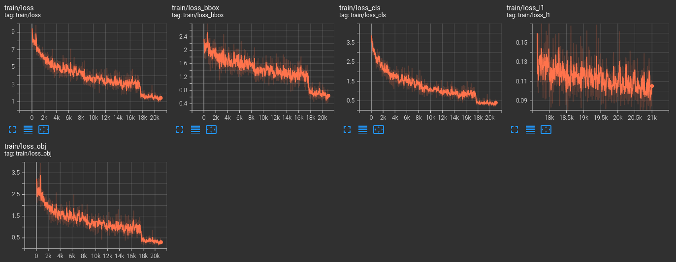
You may also observe the TensorBoard logs on your own by opening the log file from the training results directory.

Inference using the Trained YOLOX Model

Now, let’s use the trained model for carrying out inference on a few images and a video.

The inference scripts are pretty simple and straightforward.

Following is the inference_image.py code for running inference on images.

from mmdet.apis import inference_detector
from mmdet.apis import init_detector
from cfg import cfg

import argparse
import mmcv
import glob as glob
import os

# Contruct the argument parser.
parser = argparse.ArgumentParser()
parser.add_argument(
    '-i', '--input', default='input/inference_data',
    help='path to the input data'
)
parser.add_argument(
    '-w', '--weights', 
    default='outputs/yolox_l_8x8_300e_coco/best_mAP_epoch_35.pth',
    help='weight file name'
)
parser.add_argument(
    '-t', '--threshold', default=0.5, type=float,
    help='detection threshold for bounding box visualization'
)
args = vars(parser.parse_args())

# Build the model.
model = init_detector(cfg, args['weights'])

image_paths = glob.glob(f"{args['input']}/*.ppm")

for i, image_path in enumerate(image_paths):
    image = mmcv.imread(image_path)
    # Carry out the inference.
    result = inference_detector(model, image)
    # Show the results.
    frame = model.show_result(image, result, score_thr=args['threshold'])
    mmcv.imshow(frame)
    # Initialize a file name to save the reuslt.
    save_name = f"{image_path.split(os.path.sep)[-1].split('.')[0]}"
    mmcv.imwrite(frame, f"outputs/{save_name}.jpg")

It will run inference on all the images in input/inference_data directory. We can do so by executing the following command.

Note that you may have to change the path to the best mode depending on the number of epochs that you train for.

python inference_image.py --weights outputs/yolox_l_8x8_300e_coco/best_mAP_epoch_55.pth

The following are the results.

The model is performing pretty well except for a few cases. For example, it is not detecting the Ahead only label in one image and wrongly predicts a traffic light post as Stop.

Next, is the video inference script whose code is in the inference_video.py file.

from mmdet.apis import inference_detector
from mmdet.apis import init_detector
from cfg import cfg

import argparse
import mmcv
import time
import cv2

# Contruct the argument parser.
parser = argparse.ArgumentParser()
parser.add_argument(
    '-i', '--input', default='input/inference_data/video_1.mp4',
    help='path to the input file'
)
parser.add_argument(
    '-w', '--weights', 
    default='outputs/yolox_l_8x8_300e_coco/best_mAP_epoch_35.pth',
    help='weight file name'
)
parser.add_argument(
    '-t', '--threshold', default=0.5, type=float,
    help='detection threshold for bounding box visualization'
)
args = vars(parser.parse_args())

# Build the model.
model = init_detector(cfg, args['weights'])

cap = mmcv.VideoReader(args['input'])
save_name = f"{args['input'].split('/')[-1].split('.')[0]}"
fourcc = cv2.VideoWriter_fourcc(*'mp4v')
out = cv2.VideoWriter(
    f"outputs/{save_name}.mp4", fourcc, cap.fps,
    (cap.width, cap.height)
)

frame_count = 0 # To count total frames.
total_fps = 0 # To get the final frames per second.
for frame in mmcv.track_iter_progress(cap):
    # Increment frame count.
    frame_count += 1
    start_time = time.time()# Forward pass start time.
    result = inference_detector(model, frame)
    end_time = time.time() # Forward pass end time.
    # Get the fps.
    fps = 1 / (end_time - start_time)
    # Add fps to total fps.
    total_fps += fps
    show_result = model.show_result(frame, result, score_thr=args['threshold'])
    # Write the FPS on the current frame.
    cv2.putText(
        show_result, f"{fps:.3f} FPS", (15, 30), cv2.FONT_HERSHEY_SIMPLEX,
        1, (0, 0, 255), 2, cv2.LINE_AA
    )

    mmcv.imshow(show_result, 'Result', wait_time=1)
    out.write(show_result)

# Release VideoCapture()
out.release()
# Close all frames and video windows
cv2.destroyAllWindows()
# Calculate and print the average FPS
avg_fps = total_fps / frame_count
print(f"Average FPS: {avg_fps:.3f}")

Note: The video that we use is a trimmed version of the original video found here. All credit goes to the original author.

Execute the following command to run the inference.

python inference_video.py --weights outputs/yolox_l_8x8_300e_coco/best_mAP_epoch_55.pth

Following is the result.

The model is performing well here as well. The detections are not so easy here as the signs are quite small in places. It is even detecting the Road work sign correctly.

Summary and Conclusion

In this tutorial, we learned how to carry out training using MMDetection and the YOLOX model on a custom object detection dataset. I hope that you were able to learn something new from this tutorial.

If you have any doubts, thoughts, or suggestions, please leave them in the comment section. I will surely address them.

You can contact me using the Contact section. You can also find me on LinkedIn, and Twitter.