Concrete Crack Classification using Deep Learning

Computer Vision and Deep Learning are finding their way into almost every field which requires vision and learning. Starting from medical imaging to real-life industrial applications, the possibilities are endless. Analyzing and detecting structural defects in buildings is also an upcoming application of deep learning and computer vision. We can use object detection, image segmentation, and image classification depending on the problem. In this post, we will start with a simple classification problem and cover more advanced use-cases in future posts. Here, we will carry out concrete crack classification using deep learning.

This post will focus highly on the practical aspects of the problem which include:

• The dataset.
• Python code.
• Analysis of results.
• Test and inference.

Let’s check out the topics that we will cover here.

• We will start with a discussion of the dataset. In this post, we will use the Concrete Crack Image Dataset.
• Then we will move to the coding part where:
  • First, we will prepare the dataset and data loaders in the format that we need.
  • Then write the model code.
  • Next, we will prepare the training script.
  • Then we will train the model.
  • Finally, use the trained model for testing.

We will not cover the theoretical explanation of the deep learning concepts in much depth in this post.

The Concrete Crack Image Dataset

We will use the Concrete Crack Image Dataset (SDNET2018) in this post.

This dataset contains more than 56000 images of cracked and non-cracked surfaces. The surfaces in the images belong to structures like bridge decks, walls, and pavements.

The following are some of the cracked and non-cracked images from the dataset.

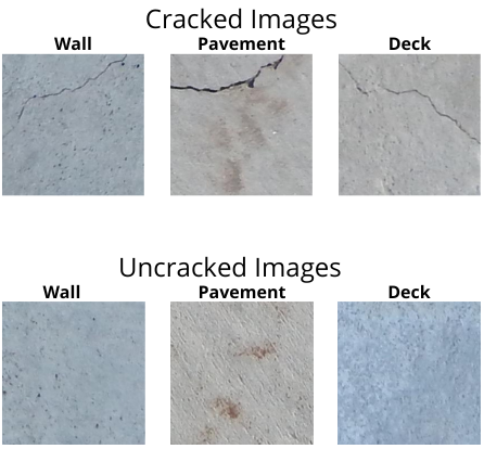
Basically, there are images belonging to two classes in this dataset. One class of images contains cracks in them and the other does not.

Right now, let’s take a look at the naming convention and directory structure of this dataset to get a better insight into it. The following is the final structure that we will be dealing with.

SDNET2018/
├── D
│   ├── CD
│   └── UD
├── P
│   ├── CP
│   └── UP
└── W
    ├── CW
    └── UW

The directories D, P, and W indicate the structure type, either bridge decks, pavements, or walls. The subdirectories contain either C or U prefixed to the structure type. Subdirectories starting with C contain images with cracks and those starting with U contain uncracked images.

Right now, you need not worry about downloading or structuring the dataset. We will directly deal with these things in the coding section.

But we need to keep in mind that this is a highly imbalanced dataset. Out of the around 56000 images, around 8400 images contain cracks in them and the rest do not. This will obviously affect the model, but to what extent, we will explore.

Directory Structure

The following block shows the directory structure for the project.

├── input
│   ├── SDNET2018
│   │   ├── D
│   │   ├── P
│   │   └── W
│   ├── test.csv
│   └── trainval.csv
├── outputs
│   ├── test_results
│   │   ├── test_image_1089.png
│   │   ...
│   │   └── test_image_99.png
│   ├── accuracy.png
│   ├── loss.png
│   └── model.pth
└── src
    ├── dataset.py
    ├── download_and_extract.py
    ├── model.py
    ├── prepare_data.py
    ├── test.py
    ├── train.py
    └── utils.py

• The input directory contains the original SDNET2018 dataset that we saw above. We will execute a simple script to download and extract this dataset. Apart from that, it contains trainval.csv and test.csv that we will generate using a data preprocessing script in the coding section.
• The outputs directory contains the output results from the test dataset as well as the accuracy & loss graphs, and the trained model.
• Finally, the src directory contains the Python code files, the details of which we will explore later in the coding section.

When downloading the zip file for this tutorial, you will get access to all the Python scripts and the trained model.

Concrete Crack Classification using Deep Learning

From here onward, we will start the coding section of the tutorial. We will cover all the necessary code in detail here.

The following are the steps that we will follow:

• Download the dataset and prepare the CSV files.
• Prepare the PyTorch datasets and data loaders.
• Prepare the training script.
• Train and test the model.

Let’s start with downloading the dataset.

Download the SDNET2018 Dataset

Before we can start training a model for concrete crack classification using deep learning, we need the dataset. The Concrete Crack Classification dataset (SDNET2018) is directly available from here. But instead of downloading it manually, let’s execute a simple script.

Note that to download the dataset using the script, you need to download the code zip files and extract them first. Please do that if you want to proceed this way. You can also download the dataset manually and structure it in the project directory in the required manner.

Download Code

The required code is available in the download_and_extract.py file. It is a simple script and we need not go into the details of it here. Just execute it from the command line/terminal in the project directory.

python download_and_extract.py

You should get an output similar to the following.

Downloading data.zip
  1%|▎                                     | 5.07M/528M [00:02<02:52, 3.03MiB/s]

Executing the script will do two things. It will download the dataset and extract it into the directory structure that we need.

Generating the Training and Testing CSV Files

To make the dataset easier to work with, we will create two CSV files. A trainval.csv and a test.csv file. They will contain two columns. One for the path to each image in the dataset and one for the corresponding label. For the labels, we consider 0 as ‘Crack Detected’ and 1 as ‘Crack Undetected’. 0 means image folder starting with ‘C’, as in ‘CW’, and 1 means image folder starting with ‘U’ as in ‘UW’.

The code to create this CSV file is present in the prepare_data.py file.

Although we will not go into the details of this code, the following block contains the entire code. Please go through it if you need to.

import pandas as pd
import os
import glob as glob

from tqdm import tqdm
from sklearn.preprocessing import LabelBinarizer

ROOT_DIR = os.path.join('..', 'input', 'SDNET2018')

# Get all the image folder paths. Structure as such so that the files inside
# the folders in `all_paths` should contain the images.
all_paths = glob.glob(os.path.join(ROOT_DIR, '*', '*'), recursive=True)
folder_paths = [x for x in all_paths if os.path.isdir(x)]
print(f"Folder paths: {folder_paths}")
print(f"Number of folders: {len(folder_paths)}")

# The class names. We will consider 0 as 'Crack Detected' 
# and 1 as 'Crack Undetected'. 0 means image folder starting with 'C', 
# as in 'CW' and 1 means image folder starting with 'U' as in 'UW'.

# Create a DataFrame
data = pd.DataFrame()

# Image formats to consider.
image_formats = ['jpg', 'JPG', 'PNG', 'png']
labels = []
counter = 0
for i, folder_path in tqdm(enumerate(folder_paths), total=len(folder_paths)):
    image_paths = os.listdir(folder_path)
    folder_name = folder_path.split(os.path.sep)[-1]
    if folder_name.startswith('C'):
        label = 0
    if folder_name.startswith('U'):
        label = 1
    # Save image paths in the DataFrame.
    for image_path in image_paths:
        if image_path.split('.')[-1] in image_formats:
            path_to_save = os.path.join(folder_path, image_path)
            data.loc[counter, 'image_path'] = path_to_save
            data.loc[counter, 'target'] = int(label)
            labels.append(label)
            counter += 1

# Shuffle the dataset.
data = data.sample(frac=1).reset_index(drop=True)

# Data to be used for training and validation.
trainval_split = 0.9

total_instances = len(data)
trainval_instances = int(total_instances*trainval_split)
test_instances = total_instances - trainval_instances 

print(f"Training and validation instances: {trainval_instances}")
print(f"Test instances: {test_instances}")
# Save as CSV file
data.iloc[:trainval_instances].to_csv(os.path.join('..', 'input', 'trainval.csv'), index=False)
data.iloc[trainval_instances:].to_csv(os.path.join('..', 'input', 'test.csv'), index=False)

Use the following command to execute the script.

python prepare_data.py

This will generate the two CSV files in the input directory.

The above figure shows a few of the rows from the trainval.csv file. The image_path column holds the image paths relative to the src directory and the target column holds the class label numbers.

The Utility and Helper Scripts

We need a few helper functions and a utility class to make our work easier throughout the project.

All of the code for this will be in the utils.py file.

Let’s start with the import statements and a function to save the trained PyTorch model.

import torch
import matplotlib
import matplotlib.pyplot as plt
import os

matplotlib.style.use('ggplot')

def save_model(epochs, model, optimizer, criterion):
    """
    Function to save the trained model to disk.
    """
    torch.save({
                'epoch': epochs,
                'model_state_dict': model.state_dict(),
                'optimizer_state_dict': optimizer.state_dict(),
                'loss': criterion,
                }, os.path.join('..', 'outputs', 'model.pth'))

The save_model function saves the trained model weights along with the number of epochs trained for, the optimizer state dictionary, and the loss function. This will help us resume training in the future if we want to.

Next, we have a simple function to save the accuracy and loss graphs to disk.

def save_plots(train_acc, valid_acc, train_loss, valid_loss):
    """
    Function to save the loss and accuracy plots to disk.
    """
    # Accuracy plots.
    plt.figure(figsize=(10, 7))
    plt.plot(
        train_acc, color='tab:blue', linestyle='-', 
        label='train accuracy'
    )
    plt.plot(
        valid_acc, color='tab:red', linestyle='-', 
        label='validataion accuracy'
    )
    plt.xlabel('Epochs')
    plt.ylabel('Accuracy')
    plt.legend()
    plt.savefig(os.path.join('..', 'outputs', 'accuracy.png'))
    
    # Loss plots.
    plt.figure(figsize=(10, 7))
    plt.plot(
        train_loss, color='tab:blue', linestyle='-', 
        label='train loss'
    )
    plt.plot(
        valid_loss, color='tab:red', linestyle='-', 
        label='validataion loss'
    )
    plt.xlabel('Epochs')
    plt.ylabel('Loss')
    plt.legend()
    plt.savefig(os.path.join('..', 'outputs', 'loss.png'))

The above function accepts the training/validation accuracy lists, and training/validation loss lists and plots the respective graphs. These graphs are stored in the outputs folder.

Finally, we have a class for the learning rate scheduler.

class LRScheduler():
    """
    Learning rate scheduler. If the validation loss does not decrease for the 
    given number of `patience` epochs, then the learning rate will decrease by
    by given `factor`.
    """
    def __init__(
        self, optimizer, patience=5, min_lr=1e-6, factor=0.1
    ):
        """
        new_lr = old_lr * factor

        :param optimizer: the optimizer we are using
        :param patience: how many epochs to wait before updating the lr
        :param min_lr: least lr value to reduce to while updating
        :param factor: factor by which the lr should be updated
        """
        self.optimizer = optimizer
        self.patience = patience
        self.min_lr = min_lr
        self.factor = factor

        self.lr_scheduler = torch.optim.lr_scheduler.ReduceLROnPlateau( 
                self.optimizer,
                mode='min',
                patience=self.patience,
                factor=self.factor,
                min_lr=self.min_lr,
                verbose=True
            )

    def __call__(self, val_loss):
        self.lr_scheduler.step(val_loss)

The LRScheduler class simply calls the ReduceLROnPlateau scheduler from torch.optim.lr_scheduler. The only reason we are again initializing this inside a custom class is to abstract it away from the training script. Basically, this will reduce the learning rate by a certain factor, when the validation loss does not improve for a certain number of epochs controlled by the patience parameter. This will help us prevent overfitting when the model starts to learn as the training progresses.

The above are all the helper functions and utility classes that we need.

Code for Dataset and DataLoaders

Let’s move on to write the code that will create the datasets and data loaders for PyTorch. We will need a custom dataset class for this.

The code for preparing the dataset will go into the dataset.py file.

The following code block deals with all the import statements.

import torch
import numpy as np
import pandas as pd
import os
import torchvision.transforms as transforms

from PIL import Image
from torch.utils.data import DataLoader, Dataset
from sklearn.model_selection import train_test_split

A few of the important modules that we import here are:

• transforms to carry out image augmentation.
• Image module from PIL to read images.
• train_test_split so that we can divide the dataset between a train and validation test.

Next, we have a custom dataset class.

# Custom dataset.
class ImageDataset(Dataset):
    def __init__(self, images, labels=None, tfms=None):
        self.X = images
        self.y = labels

        # Apply Augmentations if training.
        if tfms == 0: # If validating.
            self.aug = transforms.Compose([
                transforms.Resize((256, 256)),
                transforms.ToTensor(),
                transforms.Normalize(
                    mean=[0.485, 0.456, 0.406],
                    std=[0.229, 0.224, 0.225]
                    )
            ])
        else: # If training.
            self.aug = transforms.Compose([
                transforms.Resize((256, 256)),
                transforms.RandomHorizontalFlip(p=0.5),
                transforms.RandomVerticalFlip(p=0.5),
                transforms.RandomAdjustSharpness(sharpness_factor=2, p=0.5),
                transforms.RandomAutocontrast(p=0.5),
                transforms.RandomGrayscale(p=0.5),
                transforms.RandomRotation(45),
                transforms.ToTensor(),
                transforms.Normalize(
                    mean=[0.485, 0.456, 0.406],
                    std=[0.229, 0.224, 0.225]
                    )
            ])
         
    def __len__(self):
        return (len(self.X))
    
    def __getitem__(self, i):
        image = Image.open(self.X[i])
        image = image.convert('RGB')
        image = self.aug(image)
        label = self.y[i].astype(np.int32)
        return (
            image,
            torch.tensor(label, dtype=torch.long)
        )

It is a very simple class that first initializes the image paths (self.X) and labels (self.y). We have a tfms parameter controlling the application of augmentations depending on whether we are preparing the training or validation set. As we can see, we are applying a lot of augmentations for the training data. This is mainly to prevent overfitting by introducing more variability into the dataset.

We will be using an ImageNet pretrained model. For that reason, we are using the ImageNet normalization stats in both the training and validation transforms.

In the __getitem__ method, we simply read the image in RGB format, load the label and return both of them as tensors.

For the final part, we have the functions that will prepare the datasets and data loaders.

def get_datasets():
    # Read the data.csv file and get the image paths and labels.
    df = pd.read_csv(os.path.join('..', 'input', 'trainval.csv'))
    X = df.image_path.values # Image paths.
    y = df.target.values # Targets
    (xtrain, xtest, ytrain, ytest) = train_test_split(
        X, y,
        test_size=0.20, random_state=42
    )
    dataset_train = ImageDataset(xtrain, ytrain, tfms=1)
    dataset_valid = ImageDataset(xtest, ytest, tfms=0)
    return dataset_train, dataset_valid

def get_data_loaders(dataset_train, dataset_valid, batch_size, num_workers=0):
    """
    Prepares the training and validation data loaders.

    :param dataset_train: The training dataset.
    :param dataset_valid: The validation dataset.

    Returns the training and validation data loaders.
    """
    train_loader = DataLoader(
        dataset_train, batch_size=batch_size, 
        shuffle=True, num_workers=num_workers
    )
    valid_loader = DataLoader(
        dataset_valid, batch_size=batch_size, 
        shuffle=False, num_workers=num_workers
    )
    return train_loader, valid_loader 

The getdatasets function reads the CSV file and stores the image paths and labels in X and y variables respectively. Then we split the dataset into an 80% training set and a 20% validation set. We get the PyTorch datasets by calling the ImageDataset class on lines 63 and 64.

The get_data_loaders function accepts the training & validation datasets, the batch size, and the number of workers. It creates the respective training and validation data loaders and simply returns them.

The Deep Learning Model

We will use the MobileNetV3 Large model for concrete classification using deep learning. We will use the ImageNet pretrained weights to leverage the advantage of faster convergence.

The code for model preparation is available in the model.py file.

import torchvision.models as models
import torch.nn as nn

def build_model(pretrained=True, fine_tune=False, num_classes=10):
    if pretrained:
        print('[INFO]: Loading pre-trained weights')
    else:
        print('[INFO]: Not loading pre-trained weights')
    model = models.mobilenet_v3_large(pretrained=pretrained)

    if fine_tune:
        print('[INFO]: Fine-tuning all layers...')
        for params in model.parameters():
            params.requires_grad = True
    elif not fine_tune:
        print('[INFO]: Freezing hidden layers...')
        for params in model.parameters():
            params.requires_grad = False

    # Change the final classification head.
    model.classifier[3] = nn.Linear(in_features=1280, out_features=num_classes)
    return model

It is a pretty simple code where we load the pretrained weights based on the pretrained parameter and also decide whether to fine-tune or not based on the fine_tune parameter.

The Training Script

Now, we have reached the point to write the code for the training script.

We will write this code in the train.py file.

First, we have the import statements and the argument parsers.

import torch
import argparse
import torch.nn as nn
import torch.optim as optim
import time

from tqdm.auto import tqdm

from model import build_model
from dataset import get_datasets, get_data_loaders
from utils import save_model, save_plots, LRScheduler

# Construct the argument parser.
parser = argparse.ArgumentParser()
parser.add_argument(
    '-e', '--epochs', type=int, default=20,
    help='number of epochs to train our network for'
)
parser.add_argument(
    '-b', '--batch-size', dest='batch_size', type=int, default=32,
    help='batch size for data loaders'
)
parser.add_argument(
    '-lr', '--learning-rate', type=float,
    dest='learning_rate', default=0.001,
    help='learning rate for training the model'
)
args = vars(parser.parse_args())

We load all the custom modules that we need. For the argument parser we have the following flags:

• --epochs: To control the number of epochs to train for.
• --batch-size: To provide the batch size directly while executing the script.
• --learning-rate: We can also control the initial learning rate using this flag.

The Training and Validation Functions

We will use pretty standard PyTorch image classification functions for training and validation. The following block contains both functions.

# Training function.
def train(model, trainloader, optimizer, criterion):
    model.train()
    print('Training')
    train_running_loss = 0.0
    train_running_correct = 0
    counter = 0
    for i, data in tqdm(enumerate(trainloader), total=len(trainloader)):
        counter += 1
        image, labels = data
        image = image.to(device)
        labels = labels.to(device)
        optimizer.zero_grad()
        # Forward pass.
        outputs = model(image)
        # Calculate the loss.
        loss = criterion(outputs, labels)
        train_running_loss += loss.item()
        # Calculate the accuracy.
        _, preds = torch.max(outputs.data, 1)
        train_running_correct += (preds == labels).sum().item()
        # Backpropagation
        loss.backward()
        # Update the weights.
        optimizer.step()
    
    # Loss and accuracy for the complete epoch.
    epoch_loss = train_running_loss / counter
    # epoch_acc = 100. * (train_running_correct / len(trainloader.dataset))
    epoch_acc = 100. * (train_running_correct / len(trainloader.dataset))
    return epoch_loss, epoch_acc

# Validation function.
def validate(model, testloader, criterion):
    model.eval()
    print('Validation')
    valid_running_loss = 0.0
    valid_running_correct = 0
    counter = 0

    with torch.no_grad():
        for i, data in tqdm(enumerate(testloader), total=len(testloader)):
            counter += 1
            
            image, labels = data
            image = image.to(device)
            labels = labels.to(device)
            # Forward pass.
            outputs = model(image)
            # Calculate the loss.
            loss = criterion(outputs, labels)
            valid_running_loss += loss.item()
            # Calculate the accuracy.
            _, preds = torch.max(outputs.data, 1)
            valid_running_correct += (preds == labels).sum().item()
        
    # Loss and accuracy for the complete epoch.
    epoch_loss = valid_running_loss / counter
    epoch_acc = 100. * (valid_running_correct / len(testloader.dataset))
    return epoch_loss, epoch_acc

For both the functions, we return the loss and accuracy value for each epoch at the end.

The Main Code Block

Finally, the rest of the code is inside the main block.

if __name__ == '__main__':
    # Load the training and validation datasets.
    dataset_train, dataset_valid = get_datasets()
    print(f"[INFO]: Number of training images: {len(dataset_train)}")
    print(f"[INFO]: Number of validation images: {len(dataset_valid)}")
    # Load the training and validation data loaders.
    train_loader, valid_loader = get_data_loaders(
        dataset_train=dataset_train, 
        dataset_valid=dataset_valid,
        batch_size=args['batch_size'],
        num_workers=4
    )

    # Learning_parameters. 
    lr = args['learning_rate']
    epochs = args['epochs']
    device = ('cuda' if torch.cuda.is_available() else 'cpu')
    print(f"Computation device: {device}")
    print(f"Learning rate: {lr}")
    print(f"Epochs to train for: {epochs}\n")

    # Load the model.
    model = build_model(
        pretrained=True,
        fine_tune=True, 
        num_classes=2
    ).to(device)
    
    # Total parameters and trainable parameters.
    total_params = sum(p.numel() for p in model.parameters())
    print(f"{total_params:,} total parameters.")
    total_trainable_params = sum(
        p.numel() for p in model.parameters() if p.requires_grad)
    print(f"{total_trainable_params:,} training parameters.")

    # Optimizer.
    optimizer = optim.Adam(model.parameters(), lr=lr)
    # Loss function.
    criterion = nn.CrossEntropyLoss()
    # Initialize LR scheduler.
    lr_scheduler = LRScheduler(optimizer, patience=1, factor=0.5)

    # Lists to keep track of losses and accuracies.
    train_loss, valid_loss = [], []
    train_acc, valid_acc = [], []
    # Start the training.
    for epoch in range(epochs):
        print(f"[INFO]: Epoch {epoch+1} of {epochs}")
        train_epoch_loss, train_epoch_acc = train(
            model, 
            train_loader, 
            optimizer, 
            criterion
        )
        valid_epoch_loss, valid_epoch_acc = validate(
            model, 
            valid_loader, 
            criterion
        )
        train_loss.append(train_epoch_loss)
        valid_loss.append(valid_epoch_loss)
        train_acc.append(train_epoch_acc)
        valid_acc.append(valid_epoch_acc)
        print(f"Training loss: {train_epoch_loss:.3f}, training acc: {train_epoch_acc:.3f}")
        print(f"Validation loss: {valid_epoch_loss:.3f}, validation acc: {valid_epoch_acc:.3f}")
        lr_scheduler(valid_epoch_loss)
        print('-'*50)
        time.sleep(5)
        
    # Save the trained model weights.
    save_model(epochs, model, optimizer, criterion)
    # Save the loss and accuracy plots.
    save_plots(train_acc, valid_acc, train_loss, valid_loss)
    print('TRAINING COMPLETE')

Let’s go over some of the important parts:

• For the model initialization, we are using the pretrained weights and fine-tuning all the layers as well (line 96).
• We are initializing the learning rate scheduler on line 114. The patience is 1 and factor is 0.5. So, the learning rate will be reduced by half if the validation loss does not improve even for 1 epoch.
• After that, the for loop (from line 120) carries out the training and validation for the specified number of epochs.

In the end, we save the trained model and the accuracy & loss graphs to disk.

Execute train.py for Concrete Crack Classification using Deep Learning

Open the command line/terminal in the src directory and execute the following command.

python train.py --epochs 30 --batch-size 128

We are training for 30 epochs with a batch size of 128. If you face an Out Of Memory error, then please reduce the batch size to the maximum amount that you can fit in the memory.

The following block shows the truncated outputs.

python train.py --epochs 30 --batch-size 128
[INFO]: Number of training images: 40385
[INFO]: Number of validation images: 10097
Computation device: cuda
Learning rate: 0.001
Epochs to train for: 30

[INFO]: Loading pre-trained weights
[INFO]: Fine-tuning all layers...
4,204,594 total parameters.
4,204,594 training parameters.
[INFO]: Epoch 1 of 30
Training
100%|████████████████████████████████████████████████████████████████████████████████████████████████████████████████████████████████████████████████████████████████████████████| 316/316 [01:01<00:00,  5.14it/s]
Validation
100%|██████████████████████████████████████████████████████████████████████████████████████████████████████████████████████████████████████████████████████████████████████████████| 79/79 [00:05<00:00, 13.67it/s]
Training loss: 0.257, training acc: 91.274
Validation loss: 0.211, validation acc: 92.612
--------------------------------------------------
.
.
.
[INFO]: Epoch 29 of 30
Training
100%|████████████████████████████████████████████████████████████████████████████████████████████████████████████████████████████████████████████████████████████████████████████| 316/316 [01:00<00:00,  5.22it/s]
Validation
100%|██████████████████████████████████████████████████████████████████████████████████████████████████████████████████████████████████████████████████████████████████████████████| 79/79 [00:05<00:00, 14.04it/s]
Training loss: 0.130, training acc: 95.615
Validation loss: 0.160, validation acc: 94.850
Epoch 00029: reducing learning rate of group 0 to 3.9063e-06.
--------------------------------------------------
[INFO]: Epoch 30 of 30
Training
100%|████████████████████████████████████████████████████████████████████████████████████████████████████████████████████████████████████████████████████████████████████████████| 316/316 [01:00<00:00,  5.20it/s]
Validation
100%|██████████████████████████████████████████████████████████████████████████████████████████████████████████████████████████████████████████████████████████████████████████████| 79/79 [00:05<00:00, 14.46it/s]
Training loss: 0.127, training acc: 95.694
Validation loss: 0.160, validation acc: 94.880
--------------------------------------------------
TRAINING COMPLETE

After the final epoch, the validation loss is 0.160 and the validation accuracy is 94.880%. Looks pretty good. Let’s take a look at the graphs to get some more insights.

From the validation loss plot, it looks like the model is slightly overfitting in the final few epochs.

Testing the Trained Model for Concrete Crack Classification using Deep Learning

As we have the trained model with us now, let’s test it on all the images whose paths are available in the test.csv file. The test code is going to be pretty straightforward.

The code for testing the model is available in the test.py script.

First, we need to import all the required modules and define a few constants.

from selectors import EpollSelector
import torch
import numpy as np
import cv2
import pandas as pd
import os
import torch.nn.functional as F

from torch.utils.data import DataLoader
from tqdm.auto import tqdm
from model import build_model
from dataset import ImageDataset

# Constants and other configurations.
BATCH_SIZE = 1
DEVICE = torch.device('cuda:0' if torch.cuda.is_available() else 'cpu')
IMAGE_RESIZE = 256
NUM_WORKERS = 4
CLASS_NAMES = ['Crack Detected', 'Crack Undetected']

To create the test data loaders we will use a batch size of 1. We use the same image size as in the training, that is, 256×256. We have a CLASS_NAMES list to map the results to the class names. Index 0 will represent that a crack is detected, while index 1 will represent that a crack is not detected.

Next, we have three functions.

def denormalize(
    x, 
    mean=[0.485, 0.456, 0.406], 
    std=[0.229, 0.224, 0.225]
):
    for t, m, s in zip(x, mean, std):
        t.mul_(s).add_(m)
    return torch.clamp(x, 0, 1)

def save_test_results(tensor, target, output_class, counter):
    """
    This function will save a few test images along with the 
    ground truth label and predicted label annotated on the image.

    :param tensor: The image tensor.
    :param target: The ground truth class number.
    :param output_class: The predicted class number.
    :param counter: The test image number.
    """
    image = denormalize(tensor).cpu()
    image = image.squeeze(0).permute((1, 2, 0)).numpy()
    image = np.ascontiguousarray(image, dtype=np.float32)
    image = cv2.cvtColor(image, cv2.COLOR_RGB2BGR)
    gt = target.cpu().numpy()
    cv2.putText(
        image, f"GT: {CLASS_NAMES[int(gt)]}", 
        (5, 25), cv2.FONT_HERSHEY_SIMPLEX, 
        0.5, (0, 255, 0), 2, cv2.LINE_AA
    )
    if output_class == gt:
        color = (0, 255, 0)
    else:
        color = (0, 0, 255)
    cv2.putText(
        image, f"Pred: {CLASS_NAMES[int(output_class)]}", 
        (5, 55), cv2.FONT_HERSHEY_SIMPLEX, 
        0.5, color, 2, cv2.LINE_AA
    )
    cv2.imwrite(
        os.path.join('..', 'outputs', 'test_results', 'test_image_'+str(counter)+'.png'), 
        image*255.
    )

def test(model, testloader, DEVICE):
    """
    Function to test the trained model on the test dataset.

    :param model: The trained model.
    :param testloader: The test data loader.
    :param DEVICE: The computation device.

    Returns:
        predictions_list: List containing all the predicted class numbers.
        ground_truth_list: List containing all the ground truth class numbers.
        acc: The test accuracy.
    """
    model.eval()
    print('Testing model')
    predictions_list = []
    ground_truth_list = []
    test_running_correct = 0
    counter = 0
    with torch.no_grad():
        for i, data in tqdm(enumerate(testloader), total=len(testloader)):
            counter += 1
            image, labels = data
            image = image.to(DEVICE)
            labels = labels.to(DEVICE)

            # Forward pass.
            outputs = model(image)
            # Softmax probabilities.
            predictions = F.softmax(outputs).cpu().numpy()
            # Predicted class number.
            output_class = np.argmax(predictions)
            # Append the GT and predictions to the respective lists.
            predictions_list.append(output_class)
            ground_truth_list.append(labels.cpu().numpy())
            # Calculate the accuracy.
            _, preds = torch.max(outputs.data, 1)
            test_running_correct += (preds == labels).sum().item()

            # Save a few test images.
            if counter % 99 == 0:
                save_test_results(image, labels, output_class, counter)

    acc = 100. * (test_running_correct / len(testloader.dataset))
    return predictions_list, ground_truth_list, acc

As we will be using ImageNet normalization stats while creating the datasets, so, we will also need to denormalize them. We need this for saving the image properly to disk again with the predicted and ground-truth annotations. The denormalize function does that for us.

The save_test_results function saves an image to disk after annotating it with the ground truth and predicted label to disk.

And the test function runs the test on the entire test dataset. It returns the accuracy in the end.

Note that instead of saving all the images to disk, we save only every 99th image (line 103).

Finally, we have the main code block.

if __name__ == '__main__':
    df = pd.read_csv(os.path.join('..', 'input', 'test.csv'))
    X = df.image_path.values # Image paths.
    y = df.target.values # Targets
    dataset_test = ImageDataset(X, y, tfms=0)

    test_loader = DataLoader(
        dataset_test, batch_size=BATCH_SIZE, 
        shuffle=False, num_workers=NUM_WORKERS
    )
    checkpoint = torch.load(os.path.join('..', 'outputs', 'model.pth'))
    # Load the model.
    model = build_model(
        pretrained=False,
        fine_tune=False, 
        num_classes=2
    ).to(DEVICE)
    model.load_state_dict(checkpoint['model_state_dict'])
    predictions_list, ground_truth_list, acc = test(
        model, test_loader, DEVICE
    )
    print(f"Test accuracy: {acc:.3f}%")

We create the test data loader, load the trained model weights and call the test function.

Execute the test script using the following command.

python test.py

The following is the output.

[INFO]: Not loading pre-trained weights
[INFO]: Freezing hidden layers...
Testing model
100%|█████████████████████████████████████████████████████████████████████████████████████████████████████████████████████████████████████████████████████████████████████████| 5610/5610 [00:35<00:00, 157.98it/s]
Test accuracy: 94.973%

We get almost 95% accuracy, which is pretty nice to be fair.

Analyzing the Test Results

A few of the test results are saved to disk. Let’s check out a few of them.

The following image shows some results where the original structure did not contain any cracks and the model also predicted so.

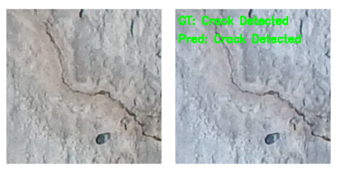
The next figure shows where the image contains cracks and the model also predicted that correctly.

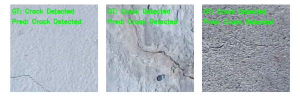
Finally, a few images where the model made mistakes.

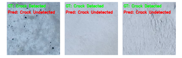
To be fair, it is pretty difficult for even a human eye to find the crack in the above images. No doubt, the model predicted them wrongly.

Further Improvements

We saw the cases where the model is making mistakes. Maybe using a bigger model like ResNet34 or ResNet50 will solve that. If you try with a larger model, try to share your results in the comment section.

Summary and Conclusion

In this post, we carried out a simple yet interesting project of concrete crack classification using deep learning. Starting from preparing the data in the appropriate format till the testing of the trained model, we followed each step. Hopefully, you found this post useful.

If you have any doubts, thoughts, or suggestions, please leave them in the comment section. I will surely address them.

You can contact me using the Contact section. You can also find me on LinkedIn, and Twitter.