In this tutorial, we will go through the concepts of Spatial Transformer Networks in deep learning and neural networks. The paper Spatial Transformer Networks was submitted by Max Jaderberg, Karen Simonyan, Andrew Zisserman, and Koray Kavukcuoglu in 2015. It addresses a very important problem in Convolutional Neural Networks and computer vision in general as well. In short, it addresses the lack of spatial invariance property in deep convolutional neural networks. We will get to know all about this in detail. We will also apply Spatial Transformer Networks using PyTorch.
What will you learn in this tutorial?
What are Spatial Transformer Networks (STNs)?
Why are they important and what problems they solve?
The problems with standard CNN.
The solution proposed by STN.
Implementing STN using PyTorch to get a strong grasp on the concept.
We will use the CIFAR10 dataset.
What are Spatial Transformer Networks (STNs)?
In general, any convolutional neural network that contains a Spatial Transformer module, we can call it a Spatial Transformer Network. So, now the question is, what are the Spatial Transformer modules?
The spatial transformer module consists of layers of neural networks that can spatially transform an image. These spatial transformations include cropping, scaling, rotations, and deformations as well.
Why do We Need STNs?
Standard convolutional neural networks are not spatially invariant to different types of input data. This means that they suffer from:
Scale / size variation in the input data.
Rotation variation in the input data.
Clutter in the input data.
CNNs perform poorly when the input data contains so much variation. One of the solutions to this is the max-pooling layer. But then again, max-pooling layers do no make the CNN invariant to large transformations in the input data.
This gives rise to the concept of Spatial Transformer Networks. In STNs, the transformer module knows where to apply the transformation to properly scale, resize, and crop and image. We can apply the STN module to the input data directly, or even to the feature maps. In simple words, we can say that the spatial transformer module acts as an attention mechanism and knows where to focus on the input data.
Taking a Look at a Simple Example
It will be much better if we see an example image.
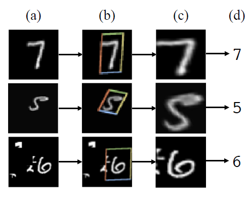
Figure 1. The working of Spatial Transformer Network on the Distorted MNIST dataset (Source).
In figure 1 we see 4 columns, (a), (b), (c), and (d). These images are from the MNIST dataset. Column (a) shows the input image to the Spatial Transformer Network. We can see that some images are deformed and some contain clutter as well. Column (b) shows where the localization network part of the STN focuses on applying the transformations. In column (c) we can see the output after the transformations. The network focuses in the digit 7, rotates the digit 5 to a more appropriate position, and crops the part of digit 6 to remove the clutter. What we see in column (d) is the classification output after we give the transformed images as an input to a standard CNN classifier.
Benefits of Spatial Transformer Networks
There are mainly three benefits of Spatial Transformer Networks which makes them easy to use.
We can include a spatial transformer module almost anywhere in an existing CNN model. Obviously, we will have to change the network architecture a bit, but that is relatively easy to do.
Spatial Transformer Networks are dynamic and flexible. We can easily train STNs with backpropagation algorithm.
They work on both, the input image data directly, and even on the feature map outputs from standard CNN layers.
The above three benefits make the usage of STNs much easier and we will also implement them using the PyTorch framework further on. Before that let’s take a brief look at the architecture of the Spatial Transformer Network.
The Architecture of Spatial Transformers
The architecture of a Spatial Transformer Network is based on three important parts.
The localization network.
The parameterized sampling grid.
And differentiable image sampling.
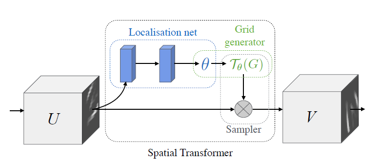
Figure 2. High level architecture of Spatial Transformer Neural Network (Source).
Figure 2 shows the overall architecture of the Spatial Transformer Network.
We will go over each of these briefly but enough to help us in coding. We will not go into much of the mathematical details as that is out of scope of this article.
The Localization Network
The localization network takes the input feature map and outputs the parameters of the spatial transformations that should be applied to the feature map. The localization network is a very simple stacking of convolutional layers.
If you take a look at figure 2, then \(U\) is the feature map input to the localization network. It outputs \(\theta\) which are the transformation parameters that are regressed from the localization network. The final regression layers are fully-connected linear layers. In figure 2, \(\mathcal{T}_\theta\) is the transformation operation using the parameters \(\theta\).
The Parameterized Sampling Grid
To get the desired output, the input feature map should be sampled from the parameterized sampling grid. The grid generator outputs the parameterized sampling grid.
Let \(G\) be the sampling grid. Now, how do we transform the input feature map to get the desirable results? Remember, we have the transformation parameters \(\theta\) and the transformation is defined by \(\mathcal{T}_\theta\). Well, we apply the transformation \(\mathcal{T}_\theta\) to the grid \(G\). That is, \(\mathcal{T}_\theta(G)\).
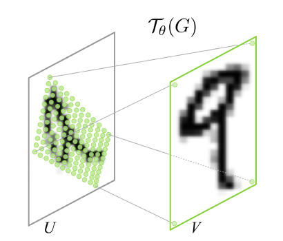
Figure 3. Warping the regular grid with affine transformation using regression parameters theta (Source).
Figure 3 shows the result of warping the regular grid with the affine transformation \(\mathcal{T}_\theta(G)\).
The output pixels lie of the grid \(G\) = \({\{G\}}_i\), where \(G_i = (x_i^t, y_i^t)\). Here, \((x_i^t, y_i^t)\) are the target coordinates.
Now, let us assume that \(\mathcal{T}_\theta\) is a 2D affine tranformation \(\mathbf{A}_\theta\). Now, the following is the whole transformation operation.
Here, \((x_i^t, y_i^t)\) are the target coordinates of the target grid in the output feature map, \((x_i^s, y_i^s)\) are the input coordinates in the input feature map, and \(\mathbf{A}_\theta\) is the affine transformation matrix.
After the sampling grid operation, we have the Differentiable Image Sampling.
Differentiable Image Sampling
This is the last part of the spatial transformer network. We have the input feature map and also the parameterized sampling grid with us now. To perform the sampling, we give the feature map \(U\) and sampling grid \(\mathcal{T}_\theta(G)\) as input to the sampler (see figure 2). The sampling kernel is applied to the source coordinates using the parameters \(\theta\) and we get the output \(V\).
There is a lot of mathematics involved in this last section which I am skipping. If you read the paper, then you will get to know them in much more detail. Although for the coding part, whatever we have covered should be enough. Still, if you want, you can give the paper a read before you move further. That will surely help you understand much of the coding easily.
From the next section, we will dive into the coding part of this tutorial.
Directory Structure and Some Prerequisites
Before you move further, make sure that you install the latest version of PyTorch (1.6 at the time of writing this) from here. This will make sure that you have all the functionalities available to follow along smoothly.
The PyTorch tutorials have a Spatial Transformer Networks Tutorial which uses the digit MNIST dataset. But we will work with the CIFAR10 dataset. This will ensure that we have a bit more complexity to handle and also we will learn how to deal with RGB (colored) images instead of grayscale images using Spatial Transformer Networks.
The input folder will contain the CIFAR10 dataset.
The outputs folder will contain all the outputs that the code generates.
In the src folder, we have the python scripts. They are model.py and train.py.
Implementing Spatial Transformer Network using PyTorch
I hope that you have set up your directory as per the above structure. From here onward, we will write the code for this tutorial. First, we will build the Spatial Transformer Network architecture. We will write that code inside the model.py file. Then we will write the code to prepare the CIFAR10 data, training, and validation function inside the train.py file.
Preparing the Spatial Transformer Network Architecture
In this section, we will write the PyTorch code for the Spatial Transformer Network Architecture. This code will go into the the model.py file inside the src folder.
First, we will write the whole network code in one code block. Then we will get to the explanation part. The following code block defines the Spatial Transformer Network Architecture.
import torch
import torch.nn as nn
import torch.nn.functional as F

class STN(nn.Module):
    def __init__(self):
        super(STN, self).__init__()
        # simple convnet classifier
        self.conv1 = nn.Conv2d(3, 6, 5)
        self.pool = nn.MaxPool2d(2, 2)
        self.conv2 = nn.Conv2d(6, 16, 5)
        self.fc1 = nn.Linear(16 * 5 * 5, 120)
        self.fc2 = nn.Linear(120, 84)
        self.fc3 = nn.Linear(84, 10)

        # spatial transformer localization network
        self.localization = nn.Sequential(
            nn.Conv2d(3, 64, kernel_size=7),
            nn.MaxPool2d(2, stride=2),
            nn.ReLU(True),
            nn.Conv2d(64, 128, kernel_size=5),
            nn.MaxPool2d(2, stride=2),
            nn.ReLU(True)
        )

        # tranformation regressor for theta
        self.fc_loc = nn.Sequential(
            nn.Linear(128*4*4, 256),
            nn.ReLU(True),
            nn.Linear(256, 3 * 2)
        )

        # initializing the weights and biases with identity transformations
        self.fc_loc[2].weight.data.zero_()
        self.fc_loc[2].bias.data.copy_(torch.tensor([1, 0, 0, 0, 1, 0],
                                                    dtype=torch.float))

    def stn(self, x):
        xs = self.localization(x)
        xs = xs.view(-1, xs.size(1)*xs.size(2)*xs.size(3))

        # calculate the transformation parameters theta
        theta = self.fc_loc(xs)
        # resize theta
        theta = theta.view(-1, 2, 3)
        # grid generator => transformation on parameters theta
        grid = F.affine_grid(theta, x.size())
        # grid sampling => applying the spatial transformations
        x = F.grid_sample(x, grid)

        return x

    def forward(self, x):
        # transform the input
        x = self.stn(x)

        # forward pass through the classifier
        x = self.pool(F.relu(self.conv1(x)))
        x = self.pool(F.relu(self.conv2(x)))
        x = x.view(-1, 16*5*5)
        x = F.relu(self.fc1(x))
        x = F.relu(self.fc2(x))
        x = self.fc3(x)
        return F.log_softmax(x, dim=1)
Explanation of the STN Architecture
I know that the above code looks complicated but I will try my best to make it as simple as possible.
Starting from line 5, we have the STN() class which contains the STN architecture.
From line 6, we have the __init__() function. In the __init__() function, from line 9 till 14, we define a simple convolutional classifier network to classify the CIFAR10 dataset images. I hope that this classification network is quite self-explanatory.
Starting from line 17 till 24, we have the Localization Network (self.localization) of the Spatial Transformer Network. First, we have a 2D convolutional layer on line 18 with 3 input channels as the CIFAR10 datasets images are colored with three channels (RGB). It is followed by max-pooling and ReLU activation. We repeat three such layers again from line 21 till 23.
Now to regress the transformation parameters \(\theta\), we need fully connected linear layers. This is exactly what the self.fc_loc module does from line 27 to 31. Now, you will see that the first linear layer’s input features are 128*4*4. This is something that we have to get through the self.localization module’s last layer’s output.
From line 34 to 35, we initialize the self.fc_loc module’s last linear layer weight and biases. We initialize them with identity transformations.
Next up, we have the stn() function from line 38. First, we get the feature maps using the self.localization module. Then we resize them and pass them onto the self.fc_loc module to get the transformation parameters theta on line 43. On line 47, we generate the parameterized sampling grid using the affine_grid() function. Finally, we apply the spatial transformations on line 49. We return the transformed feature maps on line 51.
Finally, we have the forward() function from line 53. First, we execute the stn() function to get the transformed inputs. Then, from line 57, we perform a simple forward pass through the classification network using these transformed feature maps.
Some Important Notes
I will try to answer an important question that some of you may have before moving further.
Why do we need to perform a classification after spatially transforming the inputs?
This a very valid question actually. Let’s say that we spatially transform the inputs and visualize how they look. Now what? We need some measurement criteria to determine how good the spatial transformations are, right? For that we can simply classify the transformed images from the Spatial Transformer Network instead of the original images. And with each epoch we will try to reduce the loss just as we do with general classification. The feedback from the backpropagation will force the network to return better spatial transformations with each epoch. We will also visualize in the end how with each passing epoch, the STN transforms the images spatially. I hope that this answers some of your questions.
Writing the Code to Train the STN on the CIFAR10 Dataset
This part is going to be easy. We will write the code to:
Prepare the CIFAR10 dataset.
Define the learning parameters for our Spatial Transformer Network.
Write the training and validation functions.
And finally, visualize the transformed images.
This part will not need much explanation as you will already be familiar with all the above steps. These steps are conventional to any image classification task using deep learning and PyTorch.
All the code from here onward, will go into thetrain.pyfile.
Let’s start with the imports.
import torch
import torch.optim as optim
import torch.nn as nn
import torch.nn.functional as F
import torchvision
import matplotlib.pyplot as plt
import numpy as np
import model
import imageio

from torch.utils.data import DataLoader, Dataset
from torchvision import datasets, transforms
from tqdm import tqdm
The above are all the imports that we need. We need the imageio module as we will be saving the transformed images from each epoch as a .gif file. We will analyze this short video file in the end.
Define the Learning Parameters, Transforms, and Computation Device
Next, we will define the learning parameters, the image transforms for the CIFAR10 dataset, and the computation device for training.
Initialize the Model, Optimizer, and Loss Function
Here, we will initialize the STN() model first. We will use the SGD optimizer and the CrossEntropy loss function.
# initialize the model
model = model.STN().to(device)
# initialize the optimizer
optimizer = optim.SGD(model.parameters(), lr=learning_rate)
# initilaize the loss function
criterion = nn.CrossEntropyLoss()
Define the Training Function
We will write the training function now, that is the fit() function. It is a very simple function that you must have seen a lot of times before.
# training function
def fit(model, dataloader, optimizer, criterion, train_data):
    print('Training')
    model.train()
    train_running_loss = 0.0
    train_running_correct = 0
    for i, data in tqdm(enumerate(dataloader), total=int(len(train_data)/dataloader.batch_size)):
        data, target = data[0].to(device), data[1].to(device)
        optimizer.zero_grad()
        outputs = model(data)
        loss = criterion(outputs, target)
        train_running_loss += loss.item()
        _, preds = torch.max(outputs.data, 1)
        train_running_correct += (preds == target).sum().item()
        loss.backward()
        optimizer.step()

    train_loss = train_running_loss/len(dataloader.dataset)
    train_accuracy = 100. * train_running_correct/len(dataloader.dataset)
    return train_loss, train_accuracy
Basically, for each batch of image we are:
Calculating the loss and accuracy.
Backpropagating the loss.
And updating the optimizer parameters.
Finally, for each epoch we are returning the accuracy and loss values.
Define the Loss Function
For the loss function, we will not need to backpropagate the loss or update the optimizer parameters.
# validation function
def validate(model, dataloader, optimizer, criterion, val_data):
    print('Validating')
    model.eval()
    val_running_loss = 0.0
    val_running_correct = 0
    with torch.no_grad():
        for i, data in tqdm(enumerate(dataloader), total=int(len(val_data)/dataloader.batch_size)):
            data, target = data[0].to(device), data[1].to(device)
            outputs = model(data)
            loss = criterion(outputs, target)

            val_running_loss += loss.item()
            _, preds = torch.max(outputs.data, 1)
            val_running_correct += (preds == target).sum().item()

        val_loss = val_running_loss/len(dataloader.dataset)
        val_accuracy = 100. * val_running_correct/len(dataloader.dataset)
        return val_loss, val_accuracy
Transforming the Output Images to NumPy Format
We will be saving one batch of image of each epoch from the validation set after running it through the STN() model. But we cannot save the PyTorch transformed image directly. We will first have to convert the images to NumPy format and denormalize the grid of images as well.
The following function, that is transform_to_numpy() does that for us.
def transform_to_numpy(image_grid, epoch):
    """
    This function transforms the PyTorch image grids
    into NumPy format that we will denormalize and save
    as PNG file.
    """
    image_grid = image_grid.numpy().transpose((1, 2, 0))
    mean = np.array([0.485, 0.456, 0.406])
    std = np.array([0.229, 0.224, 0.225])
    image_grid = std * image_grid + mean
    return image_grid
We can also use the save_image() function from torchvision but the above function will also help us in saving the image grids as .gif files.
Writing the Code to Get One Batch of Validation Data from the STN Model
To visualize how well our model is doing, we will pass one batch of images through the STN() model. We will save that output as a PNG file and also use the imageio module to save it as a .gif file.
images = []
def stn_grid(epoch):
    """
    This function will pass one batch of the test
    image to the STN model and get the transformed images
    after each epoch to save as PNG file and also as
    GIFFY file.
    """
    with torch.no_grad():
        data = next(iter(val_loader))[0].to(device)

        transformed_image = model.stn(data).cpu().detach()

        image_grid = torchvision.utils.make_grid(transformed_image)

        # save the grid image
        image_grid = transform_to_numpy(image_grid, epoch)
        plt.imshow(image_grid)
        plt.savefig(f"../outputs/image_{epoch}.png")
        plt.close()
        images.append(image_grid)
The images list will store all the image grids that we get from transform_to_numpy() function. We are appending those NumPy image grids to images at line 21.
Training the STN model
For training, we will just have to run a simple for loop for the number of epochs that we want to train.
# train for certain epochs
for epoch in range(epochs):
    print(f"Epoch {epoch+1} of {epochs}")
    train_epoch_loss, train_epoch_accuracy = fit(model, train_loader,
                                                 optimizer, criterion,
                                                 train_data)
    val_epoch_loss, val_epoch_accuracy = validate(model, val_loader,
                                                 optimizer, criterion,
                                                 val_data)
    print(f"Train Loss: {train_epoch_loss:.4f}, Train Acc: {train_epoch_accuracy:.2f}")
    print(f"Validation Loss: {val_epoch_loss:.4f}, Val Acc: {val_epoch_accuracy:.2f}")
    stn_grid(epoch)
Note that at line 12 we are calling the stn_grid() function to convert one batch of the validation data into NumPy format.
The final step is to save all the NumPy image grids as a .gif file using the imageio module.
That’s it. This is all the code that we need for training our STN() model.
Now, let’s execute train.py and see how well our model performs.
Executing the train.py File
Open up your terminal/command prompt and cd into the src folder. Now, execute the train.py file.
python train.py
I am showing the truncated output below.
Epoch 1 of 40
Training
0%| | 0/781 [00:00
By the end of 40 epoch, we have training accuracy of 78.52% and validation accuracy of 63.75%. The training loss is 0.0095 and validation loss 0.0184. The results are not too good. Still let’s see how well our model has spatially transformed the images.
Visualizing the Spatial Transformations Done by the STN Model
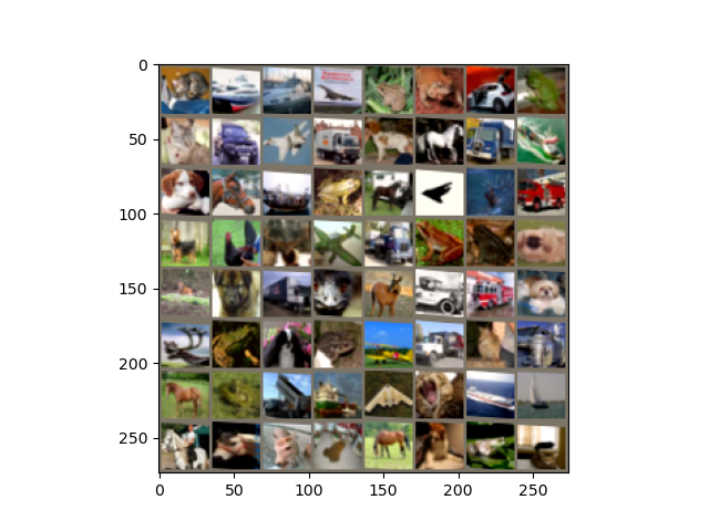
The following image shows the results after the first epoch.
Figure 4. Spatially transformed images after the first epoch.
In figure 4, we can see that the spatial transformations are not too evident. Probably this is because it is only the first epoch and the neural network has not learned much. Let’s see the results from the last epoch.
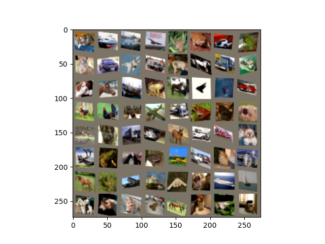
Figure 5. Result of Spatial Transformation Network after 40 epochs.
Figure 5 shows the results from the epoch 40, that is the last epoch. The spatial transformations here are very prominent. Out Spatial Transformer Network model has cropped and resized most of the images to the center. It has rotated many of the images to an orientation that it feels will be helpful. Although some of the orientations are not centered. Maybe a bit of more training will help.
Finally, let’s take a look at the .gif file that we have saved. This short video will give us the best idea of how our Spatial Transformer Network performs in each epoch.
Clip 1. Images transformed by the Spatial Transformer Neural Network after each epoch.
Clip 1 shows the images transformed by the Spatial Transformer Network after each epoch. We can see that after each epoch, the neural network is resizing, cropping, and centering the images a bit better. Still, more training will probably help even further.
Summary and Conclusion
In this tutorial, you got to learn about Spatial Transformer Networks. You got to know the basics and also implement the code for Spatial Transformer Network using PyTorch. This is a starting point and you can now start to experiment even further by improving this code. Most probably we will implement some more advanced spatial transformation techniques in future articles.
If you have any doubts, suggestions, or thoughts, then you can leave them in the comment section. I will surely address them.
You can contact me using the Contact section. You can also find me on LinkedIn, and X.
Liked it? Take a second to support Sovit Ranjan Rath on Patreon!
Hi, It’s truly inspiring.
If I have a data images (mri picture) and multi-class label images (which show where each organ is ),
can I train the data images on SNT then spatial transform the label images to make more data?
Hello le_code, I am glad that you liked the tutorial.
Yes, you can surely use STN to create different types of image data. But I would suggest that you do not do so. First of all, there is a very high chance that the STN may create distorted images from good images. Secondly, there are some better methods for image augmentation and you can also save those augmented images to disk to increase the dataset size. You can refer to this article => https://debuggercafe.com/dataset-expansion-using-image-augmentation-for-deep-learning/
You can also use GANs to create new image data, although it is really difficult to do. But if it works, it will work like a charm. I do not have a tutorial to create new image data using GAN yet. It will soon be there in the future. I hope this satisfies your queries.
This website uses cookies so that we can provide you with the best user experience possible. Cookie information is stored in your browser and performs functions such as recognising you when you return to our website and helping our team to understand which sections of the website you find most interesting and useful.
Strictly Necessary Cookies
Strictly Necessary Cookie should be enabled at all times so that we can save your preferences for cookie settings.
If you disable this cookie, we will not be able to save your preferences. This means that every time you visit this website you will need to enable or disable cookies again.


Hi, It’s truly inspiring.
If I have a data images (mri picture) and multi-class label images (which show where each organ is ),
can I train the data images on SNT then spatial transform the label images to make more data?
Best regards.
Hello le_code, I am glad that you liked the tutorial.
Yes, you can surely use STN to create different types of image data. But I would suggest that you do not do so. First of all, there is a very high chance that the STN may create distorted images from good images. Secondly, there are some better methods for image augmentation and you can also save those augmented images to disk to increase the dataset size. You can refer to this article => https://debuggercafe.com/dataset-expansion-using-image-augmentation-for-deep-learning/
You can also use GANs to create new image data, although it is really difficult to do. But if it works, it will work like a charm. I do not have a tutorial to create new image data using GAN yet. It will soon be there in the future. I hope this satisfies your queries.