Reducing Image Distortion using Spatial Transformer Network

In this article, we will learn how we can reduce distortion in images using the Spatial Transformer Network (STN) using the PyTorch deep learning library.

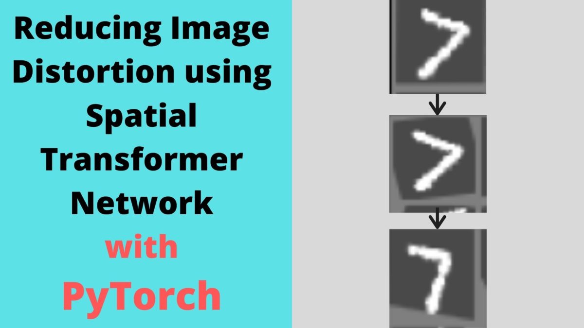
Figure 1 shows the results of applying STN to the distorted MNIST dataset. After applying STN to the distorted images, we can see that the images are spatially more plausible and readable.

If you are new to the topic of Spatial Transformer Networks, then I highly recommend that you read my previous article. You will get an introduction to Spatial Transformer Networks with all the details about the network’s architecture as well. You will also get hands-on experience by applying STNs on the CIFAR10 images and visualizing the results yourself.

Now, what new things are we going to learn in this article? Well, we will learn how to reduce distortions in images using Spatial Transformer Networks. This problem can get pretty complicated very easily. Therefore, we will start with the easiest dataset available. That is the Digit MNIST dataset which is also one of the datasets which were used for benchmarking in the original paper.

Our Approach to this Article

By now, we know that we will apply the Spatial Transformer Network to reduce distortions in the digit MNIST images.

Still, specifically, you will learn the following in this article:

• How to apply a good set of distortions and transformations to the digit MNIST images?
• Try to reproduce the results of the distortion like the original paper as much as possible.
• Apply a Spatial Transformer Network on the distorted images.
• Train the network and visualize the results.

In the original paper, the authors applied many sets of distortion to the MNIST images. Some of them are:

• Rotation.
• Rotation, translation, and scaling.
• Projective distortion.
• Elastic Distortion.

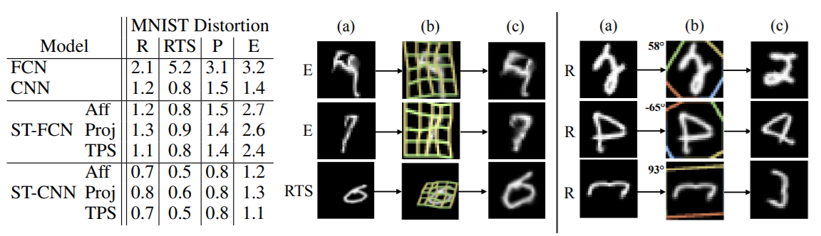
The table in the above figure (figure 2), shows the different distortions and transformations that were applied to the MNIST images. And the images on the right side show the results after applying the Spatial Transformer Network on those distorted images.

We will try to keep things a bit simple and yet try to reproduce the same transforms as the paper. We will apply the following distortions and transformations to the MNIST images.

• Random rotations: Randomly rotate the image by a certain degree. We will is the same degrees as in the original paper, which is between -45° and +45°.
• Random translation: Randomly translating the images in their own plane. We will randomly translate the images between a scale of 0.1 and 0.3. Too much translation can ruin the dataset spatially.
• Random scaling: Scaling the images randomly. The authors used scaling between 0.7 and 1.0. We will use the same too.

The above should cover a wide range of distortions to keep things a bit simple and yet provide us with an adequate challenge. This article should mainly work as a starting point to carry on such projects but on a more complicated scale further on. Now, the question is how we apply all these image transformations. Fortunately, torchvision.transforms provides the RandomAffine() function. We can use this function to apply all these transformations to the MNIST images.

Project Directory Structure and Framework

We will use the PyTorch deep learning framework in this tutorial. So, it is better if you have some experience in that. If you have the PyTorch framework already, then be sure to upgrade it to the latest version. That is PyTorch 1.6 at the time of writing this.

We will follow a simple directory structure here.

├───input
│   └───MNIST
│
├───outputs
│
└───src
    │   dataset.py
    │   model.py
    │   train.py
    │   utils.py

• The input folder will contain the MNIST dataset that we will download using torchvision.dataset module.
• All the outputs will go into the outputs folder.
• And src contains four python scripts. We will get into the details of these scripts while writing the code for each of them.

For, now just make sure that you set up your directory like the above to follow along smoothly.

Starting from the next section, we will dive into the coding part of this tutorial.

Reducing Image Distortion using Spatial Transformer Network

We will separate this part into several subsections. In each subsection, we will write the code in one of the python scripts.

Let’s start with writing some utility codes that will make our work much easier and reduce some repeatable code as well.

Writing Utility Functions

In this section, we will write the code in the utils.py file. Let’s begin with importing the modules and libraries.

import numpy
import matplotlib.pyplot as plt
import imageio
import numpy as np

Now, we will write three functions, namely, get_image_grid(), show_image(), and save_gif().

The get_image_grid() Function

The following is the code for get_image_grid() function.

def get_image_grid(image_grid):
    # unnormalize the images
    image_grid = image_grid / 2 + 0.5
    image_grid = image_grid.numpy()
    # transpose to make channels last, very important
    image_grid = np.transpose(image_grid, (1, 2, 0))
    return image_grid

It takes an input parameter, that is, image_grid which is a batch of torch tensors. This is what the function does.

• First, it unnormalizes the batch of images and converts it into NumPy format (lines 3 and 4).
• Then it transposes the image to make the dimensions as channels last (height x width x channels).
• Finally, it returns the grid image of images.

The show_image() Function

We will use the show_image() function to either visualize the images or save them to disk.

def show_image(image, DEBUG, path=None):
    plt.imshow(image)
    if DEBUG:
        plt.savefig('../outputs/distorted.png')
        plt.show()
    else:
        plt.savefig(path)
    plt.close()

It takes in three parameters, image, DEBUG, and a positional parameter path. If DEBUG is True, then we show the image and also save the image to the specified path. If DEBUG is False, then we just save the image to the path.

The save_gif() Function

We will use the imageio module to save the output images as a .gif video file. The save_gif() function will do that for us.

def save_gif(images):
    imageio.mimsave('../outputs/transformed_images.gif', images)

Next, we will move on to write the architecture of the Spatial Transformer Network.

The Spatial Transformer Network Architecture

In this section, we will write the code for the Spatial Transformer Network architecture. This architecture is the same as provided in this PyTorch tutorial. But our objective is different. We are trying to reduce image distortion using STN, whereas, in the PyTorch tutorial, the network was used on simple MNIST images. All the code here will go into model.py file.

We will not go into the details of the explanation of this architecture here. In my previous article, I provided a pretty detailed explanation of the working of the network. Including the explanation here will make the tutorial unnecessarily long. Also, that was on the colored CIFAR10 images. Please give it a read. You will learn a lot more and also find this section really easy to follow.

So, the following is the whole STN architecture.

import torch.nn as nn
import torch.nn.functional as F
import torch

class STN(nn.Module):
    def __init__(self):
        super(STN, self).__init__()
        # simple classification network to classify the MNIST images...
        # ...into 10 classes
        self.conv1 = nn.Conv2d(1, 10, kernel_size=5)
        self.conv2 = nn.Conv2d(10, 20, kernel_size=5)
        self.conv2_drop = nn.Dropout2d()
        self.fc1 = nn.Linear(320, 50)
        self.fc2 = nn.Linear(50, 10)

        # spatial transformer localization-network
        self.localization = nn.Sequential(
            nn.Conv2d(1, 8, kernel_size=7),
            nn.MaxPool2d(2, stride=2),
            nn.ReLU(True),
            nn.Conv2d(8, 10, kernel_size=5),
            nn.MaxPool2d(2, stride=2),
            nn.ReLU(True)
        )

        # to calculate the regressor parameters `theta`
        self.fc_loc = nn.Sequential(
            nn.Linear(10 * 3 * 3, 32),
            nn.ReLU(True),
            nn.Linear(32, 3 * 2)
        )

        # initialize the weights and bias with identity transformation
        self.fc_loc[2].weight.data.zero_()
        self.fc_loc[2].bias.data.copy_(torch.tensor([1, 0, 0, 0, 1, 0], dtype=torch.float))

    # spatial transformer network forward function
    def stn(self, x):
        xs = self.localization(x)
        xs = xs.view(-1, 10 * 3 * 3)
        theta = self.fc_loc(xs)
        theta = theta.view(-1, 2, 3)

        grid = F.affine_grid(theta, x.size())
        x = F.grid_sample(x, grid)

        return x

    def forward(self, x):
        # compute the spatial transformation of the input data
        x = self.stn(x)

        # forward pass for classification after the spatial transformation
        x = F.relu(F.max_pool2d(self.conv1(x), 2))
        x = F.relu(F.max_pool2d(self.conv2_drop(self.conv2(x)), 2))
        x = x.view(-1, 320)
        x = F.relu(self.fc1(x))
        x = F.dropout(x, training=self.training)
        x = self.fc2(x)
        return F.log_softmax(x, dim=1)

Some Important Things About the Network Architecture

I am including some important points about the above Spatial Transformer Network Architecture here.

• First, let’s take a look at the classification network starting from line 10. You will see that the self.conv1 on line 10 has an input channel of 1. This is because MNIST images are grayscale and have only one color channel.
• The same goes for the self.localization starting from line 17.
• Now, coming to the self.fc_loc module on line 27. You will see that the first nn.Linear() has an input feature of 10 * 3 * 3, that is 90. This number is what we get from the self.localization module’s last layer’s output. The best way to get this value is just to print the shape of the self.localization output and check what the dimensions are. Of course, if you have any other or better way to calculate it, then please let me know in the comment section. It will help the other readers too.
• The forward() function starts from line 49. First, we provide the input to the STN by calling the stn() function and passing the input as the argument on line 51. After we get the spatially transformed images, we perform the general classification on those images.

I hope that you get an intuition of how the data flows in the above network. If you have any doubts, then do ask them in the comment section. I will be glad to answer them.

Preparing the MNIST Dataset and Data Loaders

In this section, we will prepare our dataset for training the Spatial Transformer Network. We will write the code in dataset.py python file.

Let’s start with importing the modules.

import numpy as np
import torchvision
import utils
import torch

from torch.utils.data import DataLoader
from torchvision import transforms, datasets

DEBUG = True

In the above code block, you will see that we have a DEBUG variable. We will get to see its usage in a short while.

Define the Image Transforms

This part is really important. Here, we will define the image transforms that we will apply to the MNIST dataset. This forms the basis of this tutorial on what we are trying to achieve. Let’s take a look at the code.

# define the image transforms
# here, will add some distortion that we generally do not add...
# ... to the MNIST dataset, like horizontal flips, 
# random rotations, and distortions
transform = transforms.Compose([
    transforms.RandomAffine(
        degrees=(-45, 45), 
        scale=(0.7, 1.0),
        translate=(0.1, 0.3),
    ),
    transforms.ToTensor(),
    transforms.Normalize((0.1307,), (0.3081,)),
])

We are applying three different types of transformation to the images. We are using the RandomAffine() function from torchvision.transforms module.

• First, on line 7 we are rotating the images between -45° and +45°. This is what the authors used in the original paper as well.
• Then on line 8, we are scaling the images anywhere between 0.7 and 1.0 This again is according to the paper.
• On line 9, we are translating the images with parameters between 0.1 and 0.3. For translation, I did not find the values in the paper. But translation between 0.1 and 0.3 seems to work well. Too much translation can ruin the spatial position of the images in the dataset.
• Finally, we are converting the images to tensors and normalized them.

The Train/Validation Dataset and the Data Loaders

Next, we have to prepare training and validation datasets and data loaders. The following is the code for that.

# get the training and validation datasets
train_dataset = datasets.MNIST(
    root='../input',
    train=True, 
    download=True,
    transform=transform,
)
valid_dataset = datasets.MNIST(
    root='../input',
    train=False,
    download=True,
    transform=transform,
)

# prepare the training and validation datas loaders
train_data_loader = DataLoader(train_dataset, batch_size=64, shuffle=True)
valid_data_loader = DataLoader(valid_dataset, batch_size=64, shuffle=False)

For both, the train_data_loader and valid_data_loader, we are using a batch size of 64. But we are only shuffling the train_data_loader and not the valid_data_loader.

Using DEBUG to Visualize the Transformed Images

This section of the dataset.py is completely optional. Still, this will let us know what the transformed MNIST images look like. Remember, the DEBUG variable that we defined above. We are going to use it now.

Take a look at the following code block.

if DEBUG:
    sample_images, _ = iter(train_data_loader).next()
    # form a grid of images using `make_grid()`
    image_grid = torchvision.utils.make_grid(sample_images)
    grid = utils.get_image_grid(image_grid)
    utils.show_image(grid, DEBUG, path='../outputs/distorted.png')

So, this is what the code block does. If we have DEBUG as True (which we have).

• We take a sample batch from the train_data_loader.
• Then we use the make_grid() function from torchvision.utils to convert the images into a PIL image grid.
• On line 5, we call the get_image_grid() from utils which returns an unnormalized NumPy image grid.
• Finally, on line 6, we call the show_grid() function by passing the NumPy image grid and the name of the file with which to save on the disk.

The best part is, we can execute dataset.py from the terminal and get to see the distorted images. Let’s do that. Open your terminal or command prompt, cd into the src folder and execute the file.

python dataset.py

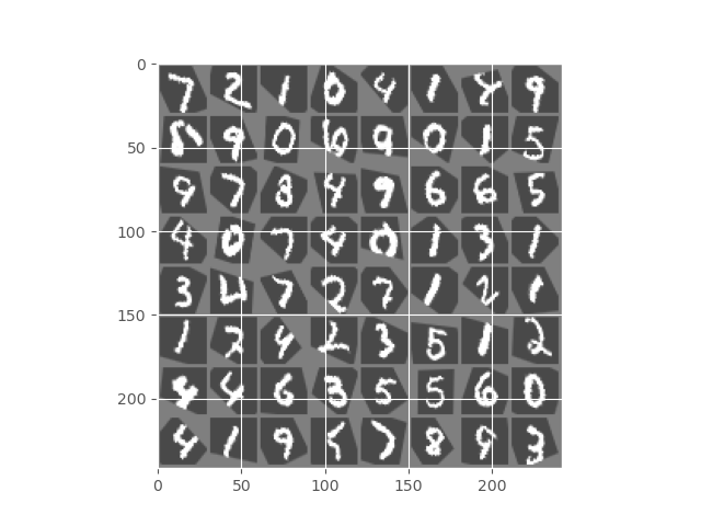
You should see an output similar to the following.

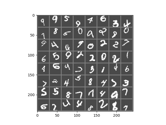
You can see that almost all the MNIST digits are somewhat distorted. Some are rotated, some are scaled, and some are translated to above or below their original position.

Now, when we train our Spatial Transformer Network on these distorted images, it should try to make the digits as much legible as possible like the original images. Hopefully, it will be able to do it.

Writing the Training Script to Train our STN

From this section onward, we will write the training script. We will write the code inside train.py file. This code part is going to be very simple. You must have seen such code a number of times before. Still, some parts will require a bit of explanation.

The following are all the modules that we need to import.

import torch
import model
import torch.optim as optim
import torch.nn as nn
import utils
import torchvision
import matplotlib.pyplot as plt
import matplotlib

from dataset import train_data_loader, valid_data_loader
from dataset import train_dataset, valid_dataset
from tqdm import tqdm

matplotlib.style.use('ggplot')

DEBUG = False

• Take a look at lines 10 and 11. We are importing train_data_loader, valid_data_loader, train_dataset, and valid_dataset from the dataset script.
• At line 16, again we have DEBUG = False. This also has its usage in this script. We will get to know further on.

Define the Computation Device and the Learning Parameters

Although not mandatory, still it is better to have a CUDA-enabled GPU for this tutorial. We will train the STN model for a large number of epochs and it may take some time to execute. It will be much faster if you have a GPU.

# computation device
device = torch.device('cuda' if torch.cuda.is_available() else 'cpu')

# learning parameters
epochs = 75
learning_rate = 0.001

We will be training our neural network model for 75 epochs. And the learning rate is going to be 0.001.

Initialize the Model, Optimizer, and Loss Function

The following code block initializes the model, optimizer, and loss function.

# initialize the model
model = model.STN().to(device)
# initialize the optimizer
optimizer = optim.SGD(model.parameters(), lr=learning_rate)
# initialize the loss function
criterion = nn.CrossEntropyLoss()

We are using the SGD() optimizer and the loss function is CrossEntropyLoss().

The Training Function

The following code block defines the training function, that is the fit() function. This is a very simple function that you must have seen many times before.

# training function
def fit(model, dataloader, optimizer, criterion, train_data):
    print('Training')
    model.train()
    train_running_loss = 0.0
    train_running_correct = 0
    for i, data in tqdm(enumerate(dataloader), total=int(len(train_data)/dataloader.batch_size)):
        data, target = data[0].to(device), data[1].to(device)
        optimizer.zero_grad()
        outputs = model(data)
        loss = criterion(outputs, target)
        train_running_loss += loss.item()
        _, preds = torch.max(outputs.data, 1)
        train_running_correct += (preds == target).sum().item()
        loss.backward()
        optimizer.step()
        
    train_loss = train_running_loss/len(dataloader.dataset)
    train_accuracy = 100. * train_running_correct/len(dataloader.dataset)    
    return train_loss, train_accuracy

• The fit() function takes 5 parameters as input. They are the neural network model, the train_data_loader, the optimizer, the loss function, and the train_dataset.
• It returns the training loss and accuracy after each epoch at line 20.

The Validation Function

The validation is almost similar to the training function. Except, we do not need to backpropagate the gradients or update the parameters.

# validation function
def validate(model, dataloader, optimizer, criterion, val_data):
    print('Validating')
    model.eval()
    val_running_loss = 0.0
    val_running_correct = 0
    with torch.no_grad():
        for i, data in tqdm(enumerate(dataloader), total=int(len(val_data)/dataloader.batch_size)):
            data, target = data[0].to(device), data[1].to(device)
            outputs = model(data)
            loss = criterion(outputs, target)
            
            val_running_loss += loss.item()
            _, preds = torch.max(outputs.data, 1)
            val_running_correct += (preds == target).sum().item()
        
        val_loss = val_running_loss/len(dataloader.dataset)
        val_accuracy = 100. * val_running_correct/len(dataloader.dataset)        
        return val_loss, val_accuracy

Function to Save the Transformed Images

We need to know whether the network is actually learning to spatially transform the images after each epoch or not. And also, if we save the output images after each epoch from the validation set, then we can analyze them later.

For this, we will write a function called stn_grid(). The following code block defines the function.

images = []
def stn_grid(epoch, data_loader):
    """
    This function will pass one batch of the test
    image to the STN model and get the transformed images
    after each epoch to save as PNG file and also as
    GIFFY file.
    """
    with torch.no_grad():
        data = next(iter(data_loader))[0].to(device)
        transformed_image = model.stn(data).cpu().detach()
        transformed_grid = torchvision.utils.make_grid(transformed_image)
        numpy_transformed = utils.get_image_grid(transformed_grid)
        # save the grid image
        utils.show_image(numpy_transformed, DEBUG, path=f"../outputs/outputs_{epoch}.png")
        images.append(numpy_transformed)

The stn_grid() function accepts two input parameters. The epoch number and a data loader which is going to be the valid_data_loader. So, what are we doing here?

• First, on line 10, we are getting the first batch of images from the valid_data_loader. On line 11, we are passing this image batch to the neural network model and saving the outputs in transformed_image.
• At line 13, we get the grid as a NumPy image.
• Line 14 calls the show_image() function from utils. Now, as DEBUG is False, so the function just saves the output to the disk and does not visualize it.
• On line 15, we append the NumPy-transformed images to the images list. We define this list at line 1 just before the stn_grid() function.

Executing the fit() and validate() Functions

We will execute the fit() and validate() functions for 75 epochs using a simple for loop.

train_loss, train_accuracy = [], []
valid_loss, valid_accuracy = [], []
# train for certain epochs
for epoch in range(epochs):
    print(f"Epoch {epoch+1} of {epochs}")
    train_epoch_loss, train_epoch_accuracy = fit(model, train_data_loader, 
                                                 optimizer, criterion, 
                                                 train_dataset)
    valid_epoch_loss, valid_epoch_accuracy = validate(model, valid_data_loader, 
                                                 optimizer, criterion, 
                                                 valid_dataset)
    print(f"Train Loss: {train_epoch_loss:.4f}, Train Acc: {train_epoch_accuracy:.2f}")
    print(f"Validation Loss: {valid_epoch_loss:.4f}, Val Acc: {valid_epoch_accuracy:.2f}")
    train_loss.append(train_epoch_loss)
    train_accuracy.append(train_epoch_accuracy)
    valid_loss.append(valid_epoch_loss)
    valid_accuracy.append(valid_epoch_accuracy)

    # call the `stn_grid()` function to save the transformed images
    stn_grid(epoch, valid_data_loader)

# save the transformed images as GIF file
utils.save_gif(images)

After each epoch, we are appending the respective losses and accuracies in train_loss, train_accuracy, and valid_loss, valid_accuracy. At line 20, we call stn_grid() to save the output images and append the NumPy grid images to images list. Finally, at line 23, we save all the images appended to images list as a .gif file to the disk.

Saving the Accuracy and Loss Plots

The final step is saving the training and accuracy plots to disk. The following code block does it.

# accuracy plots
plt.figure(figsize=(10, 7))
plt.plot(
    train_accuracy, color='green', marker='o', 
    linestyle='-', label='train accuracy'
)
plt.plot(
    valid_accuracy, color='blue', marker='o', 
    linestyle='-', label='validataion accuracy'
)
plt.xlabel('Epochs')
plt.ylabel('Accuracy')
plt.legend()
plt.savefig('../outputs/accuracy.png')
plt.show()
# loss plots
plt.figure(figsize=(10, 7))
plt.plot(
    train_loss, color='orange', marker='o', 
    linestyle='-', label='train loss'
)
plt.plot(
    valid_loss, color='red', marker='o', 
    linestyle='-', label='validataion loss'
)
plt.xlabel('Epochs')
plt.ylabel('Loss')
plt.legend()
plt.savefig('../outputs/loss.png')
plt.show()
 
print('TRAINING COMPLETE')

That is all the code we need. We can finally train our Spatial Transformer Network.

Execute the train.py File

From within the src folder in the terminal/command prompt, execute the train.py script.

python train.py

You should get output similar to the following.

Epoch 1 of 75
Training
938it [00:31, 29.50it/s]
Validating
157it [00:04, 37.97it/s]
Train Loss: 0.0361, Train Acc: 11.56
...
Epoch 75 of 75
Training
938it [00:28, 33.02it/s]
Validating
157it [00:04, 38.36it/s]
Train Loss: 0.0060, Train Acc: 88.76
Validation Loss: 0.0028, Val Acc: 94.52
TRAINING COMPLETE

Note: If you see some warnings while training, then ignore them for now. They are pretty harmless.

Analyzing the Outputs

We can see that by the end of 75 epochs, we have a training accuracy of 88.76% and a validation accuracy of 94.52%. This shows that the network is struggling to learn and classify distorted digits. Similarly, the final validation loss is less than the training loss.

The following are the saved graphical plots.

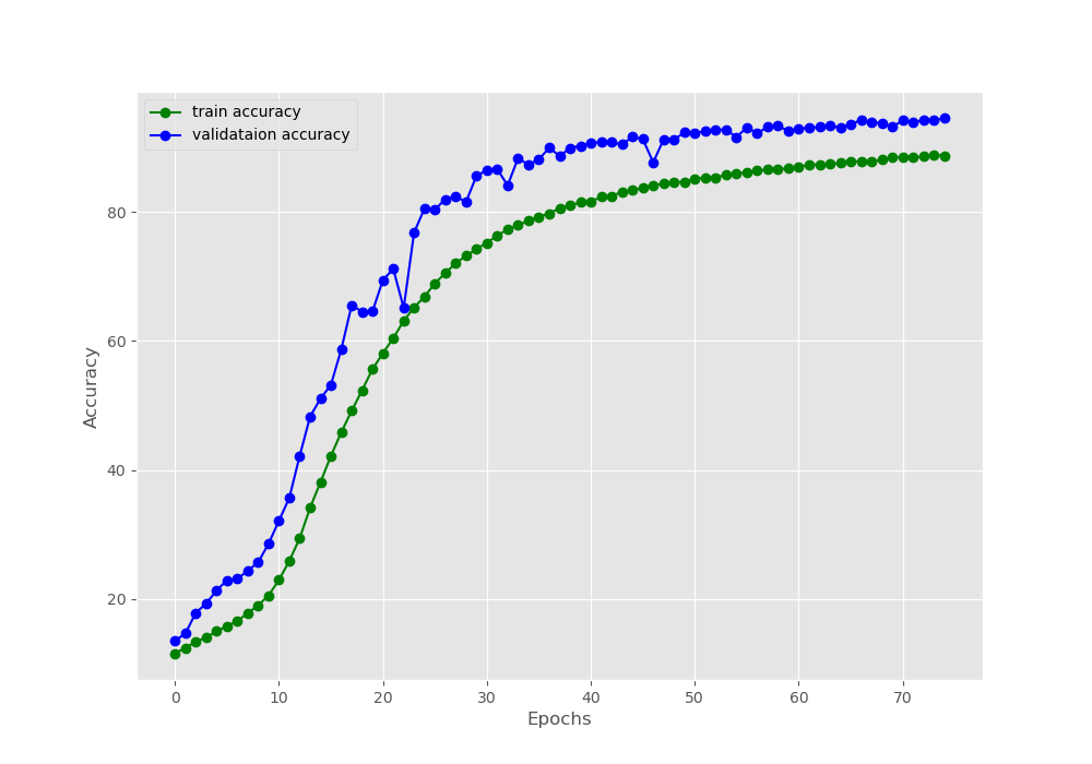
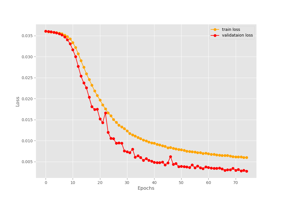
Figures 4 and 5 show the accuracy and loss plots respectively. We can see some irregularities (dips and rises) in both, the accuracy and loss plot while validating. These are most probably those images that the model finds the most difficult to classify.

Although our model performed well, most probably, increasing the network architecture size will improve the performance even more. Do try to add some more layers to the classification and spatial transformer network and post your findings in the comment section.

Analyzing the Output Images

Now, let’s take a look at the spatially transformed output images that we have saved to the disk.

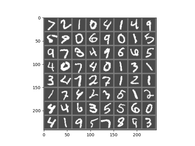
Figure 6 shows the outputs after the first epoch. We can see that almost all the images are still distorted. This is because our neural network has not started to learn anything till now.

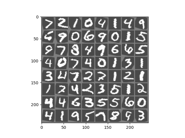
Figure 7 shows the output after 10 epochs. We can see a lot of improvements here. The Spatial Transformer Network has started to rotate and scale the digits to their original positions.

Finally, figure 8 shows the output from the final epoch. Most of the digits are transformed into a better position than they were at the beginning. Still, some digits are not quite right in their position and orientation.

In the end, let’s take a look at the short GIF that we have saved.

We can see that at the beginning the digits were not oriented properly and were distorted as well. And by the end of the training, they were much more stable and oriented in their positions. This shows that our neural network is working and improving with each epoch.

The results show the Spatial Transformer Network is doing its job properly. But most probably, bigger neural network architecture will provide even better results. Try increasing the network architecture size and tell about your findings in the comment section.

Summary and Conclusion

In this article, you learned how to use a Spatial Transformer Neural Network to reduce image distortions. You got hands-on experience and tried to reduce image distortions in the MNIST image dataset. This tutorial should provide you with adequate resources to move forward and apply your learning on a much larger dataset now.

If you have any doubts, suggestions, or thoughts, then please leave them in the comment section. I will surely address them.

You can contact me using the Contact section. You can also find me on LinkedIn, and Twitter.