Image Classification with MNIST Dataset

Updated on April 19, 2020.

The MNIST handwrttien digit data set has become the go-to guide for anyone starting out with classification in machine learning. But it is not only for students and learners. Even researchers who come up with any new classification technique also try to test it on this data. So, in this article, you will get some hands-on experience on how to tackle the MNIST data for handwritten digits.

A Bit of Background

The MNIST data set contains 70000 images of handwritten digits. This is perfect for anyone who wants to get started with image classification using Scikit-Learn library. This is because, the set is neither too big to make beginners overwhelmed, nor too small so as to discard it altogether.

As you will be the Scikit-Learn library, it is best to use its helper functions to download the data set.

Note: The following codes are based on Jupyter Notebook. It will be much easier for you to follow if you use the same as well. But there is nothing wrong in going with Python script as well.

Getting Started …

Let us first fetch the data set:

from sklearn.datasets import fetch_openml

mnist_data = fetch_openml('mnist_784', version=1)

The best part about downloading the data directly from Scikit-Learn is that it comes associated with a set of keys . Things will become very clear after you see the following code:

print(mnist_data.keys())

dict_keys(['data', 'target', 'feature_names', 'DESCR', 'details', 'categories', 'url'])

So basically, we get the `data` and target already separated. That makes the job much easier now. You can also see the description by using the DESCR. I will get down to data and target keys after the following code block:

X, y = mnist_data['data'], mnist_data['target']
print('Shape of X:', X.shape, '\n', 'Shape of y:', y.shape)

Shape of X: (70000, 784)
Shape of y: (70000,)

So the data key contains 70000 rows and 784 columns. These columns all contain the pixel intensities of the handwritten numbers ranging from 0 to 255 which are of 28 x 28 (784) images. And the target key contains all the labels from 0 to 9 corresponding to the data key pixels.

Now, let us take a look at the first few digits that are in the data set. For this, you will be using the popular matplotlib library.

import matplotlib.pyplot as plt

digit = X.iloc[0]
digit_pixels = np.array(digit).reshape(28, 28)
plt.subplot(131)
plt.imshow(digit_pixels)
plt.axis('off')

digit = X.iloc[1]
digit_pixels = np.array(digit).reshape(28, 28)
plt.subplot(132)
plt.imshow(digit_pixels)
plt.axis('off')

digit = X.iloc[2]
digit_pixels = np.array(digit).reshape(28, 28)
plt.subplot(133)
plt.imshow(digit_pixels)
plt.axis('off')

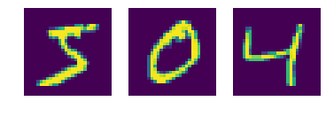
There is nothing going much in the above block of code. Still to make things a bit clearer, first I have reshaped the images from 1-D arrays to 28 x 28 matrices. Then, you will observe that I have used plt.imshow(). Actually, that takes an array image data and plots the pixels on the screen. (The pixel densities in this case).

Well, let us check whether the plots are correct or not.

y[2]

'4'

Looks like the target label of y[2] is 4 as well, but with one caveat. The target label is a string. It is better to convert the labels to integers as it will help further on in this guide.

# Changing the labels from string to integers
import numpy as np
y = y.astype(np.uint8)
y[2]

4

Now, you are all set to move ahead for the good stuff.

Separating the Training and Testing Set

Okay, your next goal is to make a separate test set which the model will not see until the test phase is reached in the process.

X_train, X_test, y_train, y_test = X[:60000], X[60000:], y[:60000], y[60000:]
print('Train Data: ', X_train, '\n', 'Test Data:', X_test, '\n',
     'Train label: ', y_train, '\n', 'Test Label: ', y_test)

Train Data:  [[0. 0. 0. ... 0. 0. 0.]  [0. 0. 0. ... 0. 0. 0.]  [0. 0. 0. ... 0. 0. 0.]  ...  [0. 0. 0. ... 0. 0. 0.]  [0. 0. 0. ... 0. 0. 0.]  [0. 0. 0. ... 0. 0. 0.]]
Test Data: [[0. 0. 0. ... 0. 0. 0.]  [0. 0. 0. ... 0. 0. 0.]  [0. 0. 0. ... 0. 0. 0.]  ...  [0. 0. 0. ... 0. 0. 0.]  [0. 0. 0. ... 0. 0. 0.]  [0. 0. 0. ... 0. 0. 0.]]
Train label:  [5 0 4 ... 5 6 8]
Test Label:  [7 2 1 ... 4 5 6]</code>

You have got your 60000 image instances as the train data and 10000 for the testing.

Training and Predicting

In this part you will be using the Stochastic Gradient Descent classifier (SGD). Scikit-Learn’s SGDClassifier is a good place to start for linear classifiers. Using the loss parameter we will see how Support Vector Machine (Linear SVM) and Logistic Regression perform for the same dataset.

Using Linear SVM

To use the Linear SVM Classifier you have to set the loss parameter to hinge. This is also set to linear SVM by default if you do not set it on your own. Let’s get to the code part:

from sklearn.linear_model import SGDClassifier

sgd_clf = SGDClassifier(loss='hinge', random_state=42)
sgd_clf.fit(X_train, y_train)

Now that you have fit your model, before moving on to testing it, let’s first see the cross-validation scores on the training data. That you will give you a very good projection of how the model performs.

from sklearn.model_selection import cross_val_score

cross_val_score(sgd_clf, X_train, y_train, cv=3, scoring='accuracy')

array([0.86872625, 0.87639382, 0.87848177])

For three-fold Cross-Validation you are getting around 87% – 88% accuracy. Not too bad, not too good either. Now let’s see the actual test scores.

score = sgd_clf.score(X_test, y_test)
score

0.8453

We are getting 84% accuracy. Okay, looks like the model generalized a bit worse than the training data.

Using Logistic Regression

Next, moving to classify using the Logistic Regression you have to set loss to log.

sgd_clf = SGDClassifier(loss='log', random_state=42)
sgd_clf.fit(X_train, y_train)

cross_val_score(sgd_clf, X_train, y_train, cv=3, scoring='accuracy')

array([0.87077584, 0.84534227, 0.87178077])

score = sgd_clf.score(X_test, y_test)
score

0.889

Interesting, although the cross-validation scores are not as good as linear SVM, but we are getting better test scores. It is not too high this time as well, but still there is a slight improvement from about 84% to about 89%.

Summary and Conclusion

You can clearly see that there is much room for improvement. You should consider using some other classifiers like the K – Nearest Neighbor (KNN). It may give better results. You can always let me know in the comment section how it performed with other classification techniques. Or maybe you can directly Contact me. Also, follow me on Twitter and Facebook to get amazing articles like this. I am always writing actively about machine learning, data science and artificial intelligence.

Before you leave – I am linking the Kaggle Kernel for this post. You can find the KNN Classification solution in this kernel. You can fork and edit it as well.