

Convolutional Neural Networks (CNN) have a come a long way in recent years. CNNs have been really beneficial for the field of deep learning for computer vision and image processing. In this article, we will be analyzing the common architectures of CNN. We will also be discussing the variants of CNN that have provided the boost to the field of deep learning.
I will try to cover the basic architectural developments of some of the well known CNNs. This article’s main aim will be to provide a good overview of the state of the art networks that researchers and machine learning practitioners use.
The Classic Network Architecture of Convolutional Neural Networks
If you are new to CNNs, then you can read one of my previous posts – Deep Learning: An Introduction to Convolutional Neural Networks.
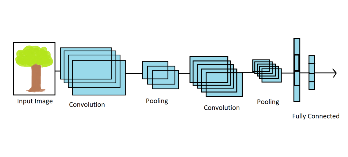
The classic CNN architectures have a few layers stacked up on top of each other. The architecture may involve a convolutional layer with activation functions, mostly ReLU, followed by a pooling layer. This process is repeated for a few layers. Then the final (top) layer involves a fully connected Dense layer with a softmax activation function.
Emergence and Development of CNN Architectures
The real emergence of convolutional neural networks for deep learning started when Yann LeCun demonstrated his LeNet – 5 in 1998. After that, over the years challenges such as ILSVRC (ImageNet Large Scale Visual Recognition Challenge) by ImageNet have constantly pushed researchers and organizations in the field to develop deeper networks.
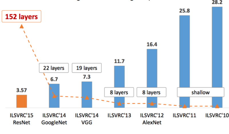
The developments have been so fast that the top-5 error percentages have dropped drastically for the ImageNet challenge.
Further on, in this article we will be discussing the following CNN architectures:
1. LeNet – 5
2. AlexNet
3. GoogLeNet
4. ResNet
LeNet – 5
Yann LeCun created LeNet – 5 in 1998. Handwritten and machine printed character recognition are the main applications of this network architecture. It has a very basic architecture, similar to that we have discussed above. The composition of layers is as following:
| Layer | Size |
| Input | 32×32 |
| Convolution | 28×28 |
| Pooling | 14×14 |
| Convolution | 10×10 |
| Pooling | 5×5 |
| Convolution | 1×1 |
| Fully Connected | 84 |
| Fully Connected (Output) | 10 |
The following image is from the original LeNet – 5 publication by Yann LeCun.
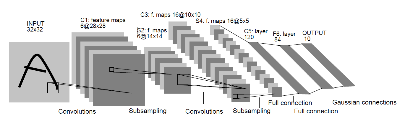
If you have worked with MNIST data set before, then the above table and image are going to very clear to you. Although the MNIST images are 28×28 in size, the input size is 32×32. According to the publication, giving larger images as inputs can really help out to distinguish the pixels for the stroke end-points of written characters at the edges. After the input layer, a series of convolutional and pooling layers follow, finally ending with a fully connected layer of size 10 (one of for each of the written digits from 0 to 9).
AlexNet
The AlexNet architecture was developed by Alex Krizhevsky, Ilya Sutskever, and Geoffrey Hinton. In 2012, AelxNet won the ILSVRC challenge with a top 5 error rate of 16%, which was almost 10% less than the runner-up model (26%).
The AlexNet network was trained on 1.2 million images at the time. As for the architecture, the following image from the publication should clear things up.
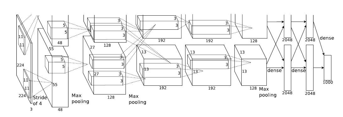
You can see that the network architecture is a bit different from a typical CNN. It consists of five convolutional layers and three fully connected dense layers, a total of eight layers. The activation function is ReLU for all the layers except the last one which is softmax activation.
To get an idea of how much complex classification AlexNet can carry out, the following is an image of inference by the network. The image is taken from the original paper.
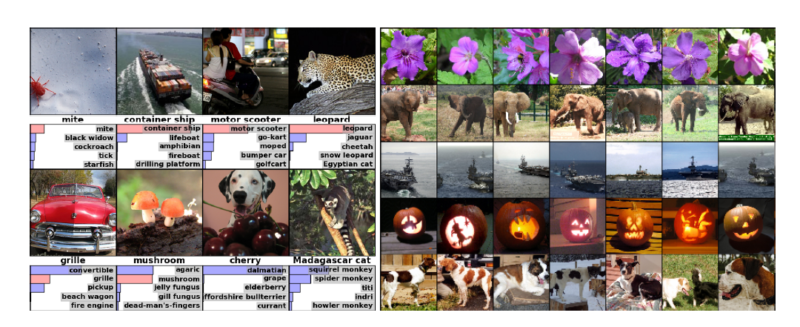
Now you must have some basic idea about the working of AlexNet. Let’s move on to the next architecture.
GoogLeNet
GoogLeNet is the winner of ILSVRC 2014. It was developed by Christian Szegedy et al. from Google and it was able to achieve below 7% top 5 error rate. Due to this it was able to beat the VGGNet architecture which was also used in that year’s challenge.
GoogLeNet is 22 layers deep and the following image will give a clear idea of the depth of the network.
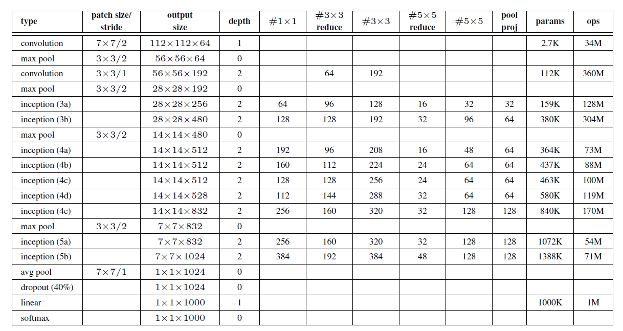
One of the interesting aspects of GoogLeNet is that it consists of Inception Modules which typically help in the desired depth of the network architecture.
The network uses Average Pooling layer instead of fully connected layer. This reduces the number of parameters drastically from 60 million (AlexNet) to just 4 million.
The first ever Inception Module was called Inception v1. In recent years, Inception Module v4 and also Inception ResNet has been developed which can obviously give even better results. These models give state of the art results on the ImageNet dataset. There are some architectural changes as well in these newer model. If you are interested in getting into more details, then give the papers a read. You will surely enjoy knowing the working of these networks.
ResNet
ResNet, short for Residual Network and was developed by Kaiming He et al. and was also the winner of ILSVRC 2015 challenge. This network achieved the top-5 error rate of 3.6% which is just mind-blowing.
The ResNet architecture consists of 152 layers in total, which is pretty deep to say the least. The following image is the architecture of ImageNet as provided in the original paper.
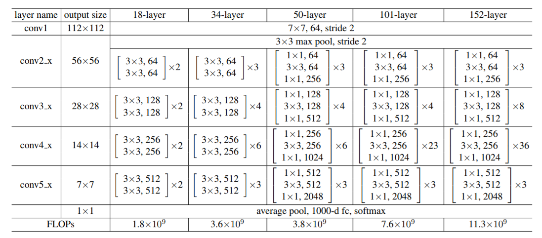
Let’s decode the image a bit as provided by the paper. So, according to the publication, the building blocks are shown in brackets. The numbers show how many of those blocks are stacked together. And conv3_1, conv4_1, conv5_1 perform downsampling with a stride of 2.
The network also uses batch normalization after each convolutional layer. A special feature of the network is skip connections, which it carries out with the use of residual blocks. This lead the network to feed the input to the current layer as well to the output of a layer which is higher up in the stack of the network.
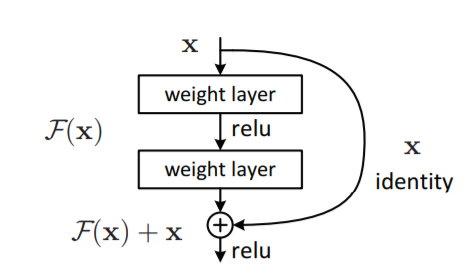
This skip connection helps to speed up training and if you add more such shortcut connections, then the model can start learning at a much faster rate than any normal neural network.
Summary and Conclusion
I hope that you got to learn the basic architectural details of CNNs. If you are interested in more detail, then I am providing a list of original publications which are really helpful.
If you liked this article, then share and give a thumbs up. Share your thoughts in the comment section and let me know if you find any inconsistencies in the article. You can follow me on Twitter, LinkedIn, and Facebook to get regular updates.

2 thoughts on “Convolutional Neural Network Architectures and Variants”