
Updated: April 8, 2020.
You must have come across numerous tutorials to distinguish between cats and dogs using deep learning. Well, then this tutorial is going to be a bit different and a whole lot interesting. In this article, we too will be using deep learning with Keras and TensorFlow for image classification. But with one difference, we will be classifying between images of wild cats, namely, golden tigers, white tigers and, mountain lions.
You can go ahead and download the project file. After extracting the file you will have the data, the pre-trained model and, also the original Jupyter Notebook.
The Directory Structure
It is not mandatory that you should use the same data as provided here. You can use your own data and by the end of this post, you will have a personal project ready. Just make sure that the folder structure of the data should be the same as provided. The following is the tree structure of the project directory.
├───.ipynb_checkpoints
├───data
│   ├───golden_tiger
│   ├───mountain_lion
│   └───white_tiger
├───images
└───logs
    ├───wild-cats-1560494714
    └───wild-cats-1560495009
We have the data directory and three sub-directories inside it. The sub-directories (golden_tiger, mountain_lion, white_tiger) contain the respective images of the wild cats. If you consider using your own data, then just replace the sub-directories with your own. The names of the sub-directories will act as labels. So, it will be better if you give intuitive names to those.
The images directory contains the test images that we will use after the model has been trained.
The logs directory contains the TensorBoard logs. We will be using TensorBoard to visualize the train and validation plots and also see the graph of the model. If you are going to use TensorBoard for the first time, then you may find this article useful.
Moreover, if you want to download new images for this tutorial, then please refer to my previous article – Create Your Own Deep Learning Image Dataset. Just one more thing. We will be using tf.keras module instead of the direct Keras API. If you find the model building codes too long, then feel free to use Keras directly. Okay, let’s start.
Loading Data and Preprocessing
The following block of code imports all the necessary packages.
# import packages
import matplotlib.pyplot as plt
import tensorflow as tf
import numpy as np
import random
import pickle
import time
import cv2
import os

from sklearn.preprocessing import LabelBinarizer
from sklearn.model_selection import train_test_split
from imutils import paths
The above code is mostly self-explanatory.
timemodule will help us to get a different timestamp for each of the TensorBoard logs so that the previous ones do not get replaced.- Using
cv2we will read the images, make necessary changes before feeding the image to the model and also visualize the predictions. - We will use
LabelBinarizerfrom Scikit-Learn to get the image labels.
Moving on, let’s get the image paths:
# path to the images
data_path = 'data'

images = []
image_labels = []

# get the image paths inside the `data` directory
image_paths = sorted(list(paths.list_images(data_path)))
# for reproducibility
random.seed(42)
# shuffle the images
random.shuffle(image_paths)
We initialize two lists, images and image_labels which will hold our images and the labels of the images respectively. For this project, we have three labels, golden_tiger, white_tiger and mountain_lion. Next, we use random.seed() for reproducibility, in case we need to run the code again. Finally, we shuffle all the images.
Now, let’s read the images and resize them using cv2. We will also append each image to the images list and the labels to the image_labels list.
for image_path in image_paths:
    # load and resize the images
    image = cv2.imread(image_path)
    image = cv2.resize(image, (128, 128))
    images.append(image)

    # get the labels from the image paths and store in `image_labels`
    image_label = image_path.split(os.path.sep)[-2]
    image_labels.append(image_label)
It is a good idea to rescale the image pixels. Rescaling is a very important factor when considering the accuracy and performance of neural networks.
# rescale the image pixels
images = np.array(images, dtype='float') / 255.0
# make `image_labels` as array
image_labels = np.array(image_labels)
Moving on, we will now split the data into train and validation test. We will be using 80% of the data for training and 20% for validation.
# divide the image data into train set and test set
(train_X, test_X, train_y, test_y) = train_test_split(images, image_labels,
                                                      test_size=0.2,
                                                      random_state=42)
The image_labels is a list of strings. To use it properly during training and inference (prediction) we need to convert those into one-hot labels.
# one-hot encode the labels
lb = LabelBinarizer()
train_y = lb.fit_transform(train_y)
test_y = lb.fit_transform(test_y)
So, now for golden_tiger, we will have [1, 0, 0]. This means that the image is true for golden_tiger only (hence, the 1). Similarly, it will be [0, 1, 0], [0, 0, 1] for mountain_lion and white_tiger respectively.
Next, we will insert the code image augmentation generator. This will provide our model with a lot of different cases to learn while training. Hopefully, this step will help in achieving better accuracy.
# generator for image augmentation
image_aug = tf.keras.preprocessing.image.ImageDataGenerator(rotation_range=30, shear_range=0.2,
    zoom_range=0.2, height_shift_range=0.2, width_shift_range=0.2,
    horizontal_flip=True, fill_mode='nearest')
For data augmentation, we are using the ImageDataGenerator from tf.keras module.
Building the Model
Now, its time to build our model. Frankly, the model does have a lot of layers. Let’s insert the code fist, then I will move on to explain the layers.
# build the model
model = tf.keras.models.Sequential()
input_shape = (128, 128, 3)

model.add(tf.keras.layers.Conv2D(32, (3, 3), padding='same',
            activation='relu', input_shape=input_shape))
model.add(tf.keras.layers.BatchNormalization(axis=-1))
model.add(tf.keras.layers.MaxPooling2D(pool_size=(2, 2)))
model.add(tf.keras.layers.Dropout(0.2))

model.add(tf.keras.layers.Conv2D(64, (3, 3), padding='same',
                                 activation='relu'))
model.add(tf.keras.layers.BatchNormalization(axis=-1))
model.add(tf.keras.layers.Conv2D(64, (3, 3), padding='same',
                                 activation='relu'))
model.add(tf.keras.layers.BatchNormalization(axis=-1))
model.add(tf.keras.layers.MaxPooling2D(pool_size=(2, 2)))
model.add(tf.keras.layers.Dropout(0.2))

model.add(tf.keras.layers.Conv2D(128, (3, 3), padding='same',
                                 activation='relu'))
model.add(tf.keras.layers.BatchNormalization(axis=-1))
model.add(tf.keras.layers.Conv2D(128, (3, 3), padding='same',
                                 activation='relu'))
model.add(tf.keras.layers.BatchNormalization(axis=-1))
model.add(tf.keras.layers.Conv2D(128, (3, 3), padding='same',
                                 activation='relu'))
model.add(tf.keras.layers.BatchNormalization(axis=-1))
model.add(tf.keras.layers.MaxPooling2D(pool_size=(2, 2)))
model.add(tf.keras.layers.Dropout(0.2))

model.add(tf.keras.layers.Flatten())
model.add(tf.keras.layers.Dense(512, activation='relu'))
model.add(tf.keras.layers.BatchNormalization())
model.add(tf.keras.layers.Dropout(0.2))

model.add(tf.keras.layers.Dense(len(lb.classes_), activation='softmax'))
First of all, we are using the Sequntial() API to build the model. Secondly, the we have given the input shape as (128, 128, 3) for the height, width and channels. So, it is a channels last input shape.
Now, moving on to the actual layers, we are using Conv2D with relu activation function and padding=same. For the first convolutional layer we have given the output dimensionality as 32. Then we gradually increase it to 64 and 128. Each of the Conv2D layer is having its own BatchNormalization layer as well. The axis is -1 as we are using channels last. Then we have the MaxPooling layer with pool_size=(2, 2) and Dropout layer with a rate of 0.2.
In the model, the only exceptions are the last hidden layer and the output layer. For the last hidden layer we are using Dense with 512 dimensionality. The output layer is using softmax activation function and the output dimensionality is len(lb.classes). That would amount to 3 as we have 3 classes in total.
Now, we are going to create a TensorBoard callback to save the training logs.
NAME = 'wild-cats-{}'.format(int(time.time())) # to save different tensorboard logs each time

tensorboard = tf.keras.callbacks.TensorBoard(log_dir='logs/{}'.format(NAME))
Compiling and Running the Model
In this part, we are going to define the optimizer, compile the model and train it using fit_generator. We will be using fit_generator() instead of fit() as we have an ImageDataGenerator() in the pipeline for augmenting the images.
optimizer = tf.keras.optimizers.Adam(lr=0.01)
model.compile(loss='categorical_crossentropy', optimizer=optimizer,
              metrics=['accuracy'])

history = model.fit_generator(image_aug.flow(train_X, train_y,
                                             batch_size=32),
                              validation_data=(test_X, test_y),
                              steps_per_epoch=len(train_X) // 32,
                              epochs=50, callbacks=[tensorboard])
Saving the Model
It is always a good idea to save the model weights after training. Here, we will be saving the trained model as well as the labels as a pickle file.
model.save('conv2d.model')
f = open('conv2d_lb.pickle', 'wb')
f.write(pickle.dumps(lb))
f.close()
Plotting and TensorBoard Visualization
Before we move on to the inference stage let’s see all the accuracies and losses in a single plot. That would help in comparing them in a better way.
num_epochs = np.arange(0, 50)
plt.figure(dpi=300)
plt.plot(num_epochs, history.history['loss'], label='train_loss', c='red')
plt.plot(num_epochs, history.history['val_loss'],
    label='val_loss', c='orange')
plt.plot(num_epochs, history.history['acc'], label='train_acc', c='green')
plt.plot(num_epochs, history.history['val_acc'],
    label='val_acc', c='blue')
plt.title('Training Loss and Accuracy')
plt.xlabel('Epoch')
plt.ylabel('Loss/Accuracy')
plt.legend()
plt.savefig('plot.png')
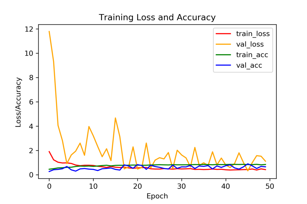
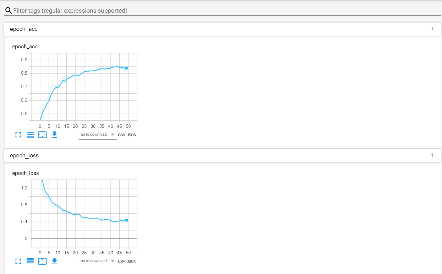
The validation loss does not look very stable. There can be numerous reasons for this. One of the reasons is the similarity between the images and also the small number of images. You can also get a TensorBoard visualization of the plots and the model graph as well. In the command line (in the project directory), type the following:
tensorboard --logdir=logs/
Then go to http://localhost:6006/#scalars .
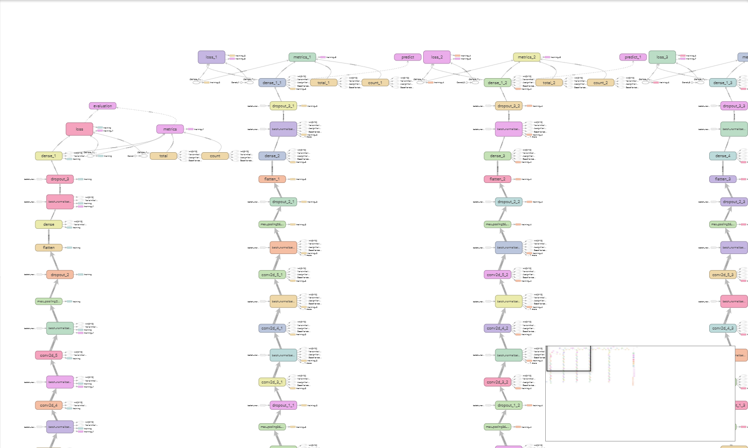
You can also click on the GRAPHS tab to see the model graph.
Predicting
The code that follows can be run fully independently without running any of the previous code after you have completed the training part. So, you can always predict on new images only by executing the following code snippets. If you want, you can also save this part in a predict.py python file which you can run independently without opening the Jupyter Notebook.
Let’s load one of the test images, scale the pixels and reshape it as well:
# load the test image
image = cv2.imread('images/golden.jpg')
output = image.copy()
image = cv2.resize(image, (128, 128))

# scale the pixels
image = image.astype('float') / 255.0

image = image.reshape((1, image.shape[0], image.shape[1], image.shape[2]))
Loading the model and the label binarizer.
model = tf.keras.models.load_model('conv2d.model')
lb = pickle.loads(open('conv2d_lb.pickle', 'rb').read())
Now, predicting and getting the class labels.
# predict
preds = model.predict(image)

# get the class label
max_label = preds.argmax(axis=1)[0]
print('PREDICTIONS: \n', preds)
print('PREDICTION ARGMAX: ', max_label)
label = lb.classes_[max_label]
PREDICTIONS: [[9.2370689e-01 2.5450445e-06 7.6290570e-02]]
PREDICTION ARGMAX: 0
Finally, let’s see the predictions.
# class label along with the probability
text = '{}: {:.2f}%'.format(label, preds[0][max_label] * 100)
cv2.putText(output, text, (10, 30), cv2.FONT_HERSHEY_SIMPLEX, 0.7, (0, 0, 255), 2)
cv2.imshow('image', output)
cv2.waitKey(0)
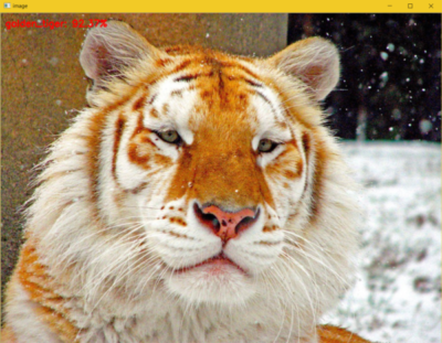
Our model is predicting the image as golden_tiger with 92.3% accuracy, which is fairly good. But when you predict for the other images, you may sometimes get wrong results. One reason is that our data set is fairly small (only about 350 images in total for each class). You can always try to find more images for better training. Other times you may find that if white tiger image has a yellowish hue (maybe sunrise), then also the model is predicting the image as golden_tiger or maybe mountain_lion. Adding a variety of images covering different scenes appears to be the only solution here. You should surely try out these.
Conclusion
In this tutorial, you learned how to build your own image classifier using TensorFlow and Keras. From here on, you can try training the model on different images.
Again, you can download the files here:
Be sure to share your thoughts in the comment section and subscribe to the website as well. Don’t forget to give a Thumbs Up You can also follow me on Twitter, Facebook, and LinkedIn.
