Keras Deep Learning with TensorBoard Visualization

Many of the times, after building a model we tend to visualize the accuracy and validation plots manually with Matplotlib (or any other) visualization library. But there is a better way to do it. We can easily visualize the plots using TensorBoard which provides a beautiful and interactive environment by default. In this article, you will be building a Keras Deep Learning model for the MNIST handwritten digits. Then you will get to know how to effectively visualize plots with TensorBoard.

Prerequisites: It is better to have some prior knowledge of Keras and Deep Learning.

Let’s Get Started

We import all the requirements first:

import tensorflow as tf
import numpy as np
import time
import pickle

from tensorflow import keras
from tensorflow.keras.callbacks import TensorBoard
from tensorflow.keras.callbacks import EarlyStopping
from tensorflow.keras.callbacks import ModelCheckpoint
from tensorflow.keras import models

The next block of code downloads the data, normalizes it and divides the data into train and validation set:

(X_train, y_train), (X_test, y_test) = tf.keras.datasets.mnist.load_data()
X_train = X_train.astype(np.float32) / 255.0
X_test = X_test.astype(np.float32) / 255.0
y_train = y_train.astype(np.int32)
y_test = y_test.astype(np.int32)
X_valid, X_train = X_train[:5000], X_train[5000:]
y_valid, y_train = y_train[:5000], y_train[5000:]

The above code, after downloading the data normalizes the features (pixel densities) by converting to `float32` and dividing them by 255.0. Then we convert the labels to `int32`. As usual, the MNIST data contains 60000 instances in the train set and 10000 instances in the test set. Out of the 60000 training instances, we will be using 55000 for training and 5000 for validating.

Now, we can define number of inputs. That will be equal to the number of features in a single row (28). We will use two hidden layers. One hidden layer with 300 neurons and the other with 100. The output layer will contain 10 neurons, one for each of 10 number (from 0 to 9).

n_inputs = 28
n_hidden1 = 300
n_hidden2 = 100
n_outputs = 10

That’s done. Now, let’s define the model. We will use the `Sequential()` model API.

model = tf.keras.Sequential()
model.add(tf.keras.layers.Flatten(input_shape=(n_inputs, n_inputs)))
model.add(tf.keras.layers.Dense(n_hidden1, activation=tf.nn.relu))
model.add(tf.keras.layers.Dense(n_hidden2, activation=tf.nn.relu))
model.add(tf.keras.layers.Dense(n_outputs, activation=tf.nn.softmax))

The `Flatten()` function first takes the 2D list of features (28, 28) and flattens them into a single row. Then we are using three Dense() layers. The first two are for the two hidden layers which we have defined above. The activation function is relu(Rectified Linear Unit) for these two hidden layers. The final dense layer is for the outputs with `softmax` activation function.

Okay, that’s done. Before moving further into model compilation and fitting we will define the code for early stopping and model checkpoint.

Early stopping will help to stop the training when there is no improvement in the accuracy for a certain number of steps. And model checkpoint will help us to save the best model. We have already imported EarlyStopping and ModelCheckpoint at the beginning.

NAME = 'mnist-{}'.format(int(time.time())) # to save different tensorboard logs each time

tensorboard = TensorBoard(log_dir='logs/{}'.format(NAME))

# early stopping
stop = EarlyStopping(monitor='val_loss', mode='min', verbose=1, patience=10)
# define checkpoints
checkpoint = ModelCheckpoint('best_model.h5', monitor='val_acc', mode='max', verbose=1, save_best_only=True)

The TensorBoard logs will be saved inside the logs/ directory where the project is located. Each time you train the model, the logs will have a different timestamp associated with the NAME. This will prevent the overwriting of previous logs (so that we can compare the different results).

For early stopping, we have defined patience=10. The model will stop training when there is no improvement in validation accuracy for 10 epochs.

We are ready to compile and train the model.

model.compile(optimizer='adam', 
              loss='sparse_categorical_crossentropy', 
              metrics=['accuracy'])

history = model.fit(X_train, y_train, 
                    epochs=100, 
                    validation_data=(X_valid, y_valid), 
                    verbose=1, 
                    callbacks=[tensorboard, stop, checkpoint])

You should be getting somewhere around 97% to 98% validation accuracy. We can now evaluate the model on the test set:

accuracy = model.evaluate(X_test, y_test)

print('Accuracy: ', accuracy[1])

Accuracy:  0.9785 

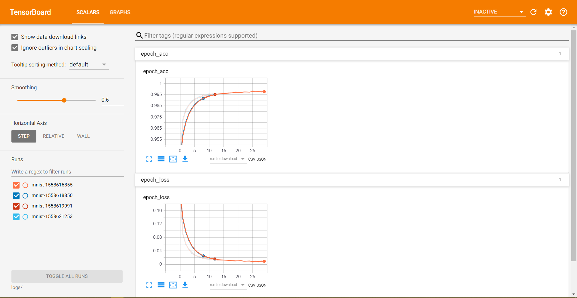
We are getting pretty good results. But we are not done here. Let’s visualize the plots on TensorBoard now. Open your terminal, then migrate to your project directory and type the following:

tensorboard --logdir=logs/

You should see something like this:

TensorBoard 1.13.1 at http://MSI:6006

You can now go to the address given. But if you get a connection refused error, then you try http://localhost:6006/ instead. It should work now. You should be able to visualize the plots.

Now you are all set to train your models, apply the techniques on new projects and that too with interactive visualization.

Conclusion

I hope that you liked the post. Please share and give a thumbs up. You can follow me on Twitter, Facebook, and LinkedIn to get notified about new content. And don’t forget to subscribe to the newsletter.