Traffic Sign Recognition using Neural Networks

Computer Vision and Deep Learning together have given some novel solutions to many of the real world problems. And automatic traffic sign recognition is one of them. Recognizing traffic signs is one of the most important aspects when considering road safety and automated driving. Manual detection, classification, and hard coding are not possible when visualizing hundreds of miles of road. In this case, computer vision combined with deep learning and Convolutional Neural Networks can help a lot.

In this article, we will be using CNN to recognize traffic signs. We will use Sequential() API along with tf.keras to build the model.

Prerequisites

You should be familiar with basic Python code along with some experience in Keras, TensorFlow and Convolutional Neural Networks in general. If you have been using Keras and TensorFlow for some time now, then it will be really easy for you to follow along.

The Data

The data is taken from GTSRB (The German Traffic Sign Recognition Benchmark). It is one of the best archives to get traffic sign images. You can download the dataset here. Scroll down to the dataset table and download the GTSRB_Final_Training_Images.zip. file.

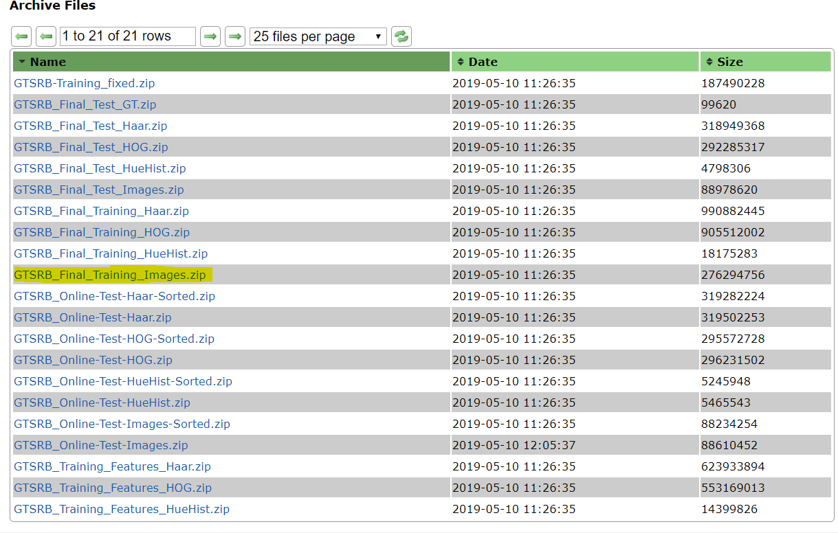
After you unzip the file, the folder structure is as follows:
GTSRB/Final_Training/Images/00007/ , where 00007/ contains images of a particular traffic sign. The CSV file inside the directory contains the ClassId 7 which corresponds to the directory name. There are 43 classes (directories) like this, ranging from 00001/ to 00042/. Make yourself familiar with the directory structure and you will be good to follow along.

Okay, now we are ready to move into the code part.

Importing Required Packages

Let’s import all the required packages that we will be needing to complete this project.

import matplotlib.pyplot as plt
import tensorflow as tf
import numpy as np
import time
import glob 
import cv2
import os

from sklearn.model_selection import train_test_split
from skimage.color import rgb2grey

Most of the packages are self-explainable, except a few.

• We will use the glob package to do path matching for the images.
• rgb2grey from skimage.color will help us to convert the colored images into grey scale images. This is particularly required as all the images are not perfectly clear. Some may have more contrast, while in other images the lighting may not be so good.

There are 43 classes in total. We can define the number of classes and also call a re-seed generator as well.

NUM_CLASSES = 43
np.random.seed(42)

Loading and Preprocessing the Data

In this section, we will load the data and convert them into grey-scale images. After that, we will rescale the pixel values so that they all fall within the range [0.0, 255.0]. Also, we will resize the images to 32×32 size. Finally, we will one-hot encode the labels.

# path to the images
data_path = 'GTSRB_Final_Training_Images/GTSRB/Final_Training/Images'

images = []
image_labels = []

# get the image paths
for i in range(NUM_CLASSES):
    image_path = data_path + '/' + format(i, '05d') + '/'
    for img in glob.glob(image_path + '*.ppm'):
        image = cv2.imread(img)
        image = rgb2grey(image)
        image = (image / 255.0) # rescale
        image = cv2.resize(image, (32, 32)) #resize
        images.append(image)
        
        # create the image labels and one-hot encode them
        labels = np.zeros((NUM_CLASSES, ), dtype=np.float32)
        labels[i] = 1.0
        image_labels.append(labels)

images = np.stack([img[:, :, np.newaxis] for img in images], axis=0).astype(np.float32)
image_labels = np.matrix(image_labels).astype(np.float32)

So, after one-hot encoding the labels, every image will have 43 labels, all zeros except for the corresponding image label which will be 1. It will become more clear after you see the following output.

plt.imshow(images[45, :, :, :].reshape(32, 32), cmap='gray')
print(image_labels[45, :])

[[1. 0. 0. 0. 0. 0. 0. 0. 0. 0. 0. 0. 0. 0. 0. 0. 0. 0. 0. 0. 0. 0. 0. 0.   0. 0. 0. 0. 0. 0. 0. 0. 0. 0. 0. 0. 0. 0. 0. 0. 0. 0. 0.]]

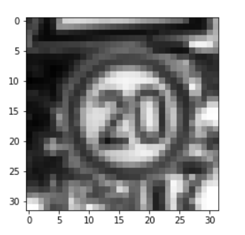
The above output is for the 45th image, which is in the first directory. Therefore, only the first label is 1 and all others are zero.

For assurance, let’s print the number of images and their shape.

print(images.shape)
print(len(images))

(39209, 32, 32, 1) 
39209

Alright, let’s move ahead and divide our data into train and test set.

Prepare Train and Test Data

We will be using 20% of the images for validation for testing and the rest for training.

# divide the data into train and test set
(train_X, test_X, train_y, test_y) = train_test_split(images, image_labels, 
                                                      test_size=0.2, 
                                                      random_state=42)
print(train_X.shape)
print(train_y.shape)
print(test_X.shape)
print(test_y.shape)

(31367, 32, 32, 1) 
(31367, 43) 
(7842, 32, 32, 1) 
(7842, 43)

Build the Model

We are all set to build our ConvNet model.

Here, we will use the Sequential() API from tf.keras to build the model.

The input shape has a channel dimension of 1 as the images are grey scale. There are three Conv2D() layers with output dimensions of 32, 64 and 128 respectively. The activation function is ReLU and padding is same. The axis is -1 for BatchNormalization() as the inputs are channels_last. Also we are using Dropout() of 0.2 for each of the Conv2D(). The Maxpooling2D() has pool_size() of (2, 2).

At last we flatten the images and use a Dense() layer with output dimension of 512 and ReLU activation. Here, the dropout rate is 0.4 and the final Dense() layer has output dimensionality of 43 for each of the 43 classes with softmax activation funtion.

# initialize the model
model = tf.keras.models.Sequential()
input_shape = (32, 32, 1) # grey-scale images of 32x32

model.add(tf.keras.layers.Conv2D(32, (5, 5), padding='same', 
            activation='relu', input_shape=input_shape))
model.add(tf.keras.layers.BatchNormalization(axis=-1))      
model.add(tf.keras.layers.MaxPooling2D(pool_size=(2, 2)))
model.add(tf.keras.layers.Dropout(0.2))
        
model.add(tf.keras.layers.Conv2D(64, (5, 5), padding='same', 
                                 activation='relu'))
model.add(tf.keras.layers.BatchNormalization(axis=-1))
model.add(tf.keras.layers.Conv2D(128, (5, 5), padding='same', 
                                 activation='relu'))
model.add(tf.keras.layers.BatchNormalization(axis=-1))
model.add(tf.keras.layers.MaxPooling2D(pool_size=(2, 2)))
model.add(tf.keras.layers.Dropout(0.2))

model.add(tf.keras.layers.Flatten())
model.add(tf.keras.layers.Dense(512, activation='relu'))
model.add(tf.keras.layers.BatchNormalization())
model.add(tf.keras.layers.Dropout(0.4))

model.add(tf.keras.layers.Dense(43, activation='softmax'))

Compile and Run the Model

We will use Adam() optimizer with a learning rate of 0.001. The loss function is going to be categorical_crossentropy and metrics will be accuracy. The model will run for 10 epochs.

optimizer = tf.keras.optimizers.Adam(lr=0.001)
model.compile(loss='categorical_crossentropy', optimizer=optimizer, 
              metrics=['accuracy'])

history = model.fit(train_X, train_y, 
                   validation_data=(test_X, test_y),
                   epochs=10)

By the end of 10 epochs, you should easily be getting above 97% accuracy which is fairly good for a first try.

Accuracy and Loss Plots

Let’s see how our model performed epoch wise. The following plot should give a clear idea.

num_epochs = np.arange(0, 10)
plt.figure(dpi=300)
plt.plot(num_epochs, history.history['loss'], label='train_loss', c='red')
plt.plot(num_epochs, history.history['val_loss'], 
    label='val_loss', c='orange')
plt.plot(num_epochs, history.history['acc'], label='train_acc', c='green')
plt.plot(num_epochs, history.history['val_acc'], 
    label='val_acc', c='blue')
plt.title('Training Loss and Accuracy')
plt.xlabel('Epoch')
plt.ylabel('Loss/Accuracy')
plt.legend()
plt.savefig('plot.png')

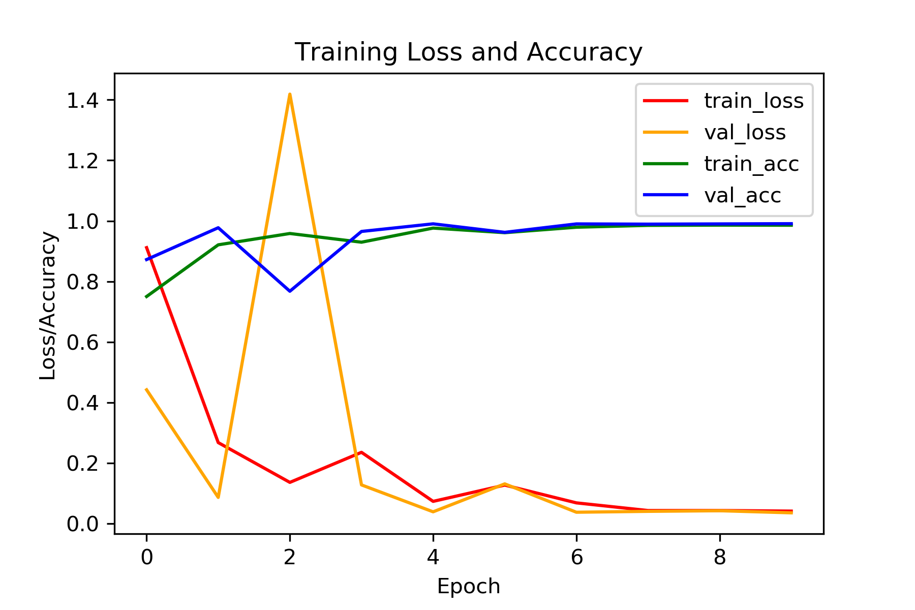
The val_loss was a bit high in the second epoch. But after that it was almost in sync with the train_loss and also quite low. By the end we are getting around 0.03 val_loss and 0.99 val_acc which is pretty good for a first try.

Summary and Conclusion

Now you have a model that can recognize traffic signs with great accuracy. You can use this model for your own project or further train this on more images with different lighting and weather conditions.

I hope that you gained some good insights from this tutorial. If so, then give a thumbs up and share this with others. You can follow me on Twitter, LinkedIn, and Facebook to get regular updates as well. Subscribe to the website and you will get awesome content in your mailbox regularly. Also, don’t forget to leave your thoughts in the comment section and do let me know if you find any inconsistencies in this article.