LeNet-5: A Practical Approach

Updated on 21 April, 2020.

LeNet – 5 is a great way to start learning practical approaches of Convolutional Neural Networks and computer vision. The LeNet – 5 architecture was introduced by Yann LeCun, Leon Bottou, Yoshua Bengio and Patrick Haffner in 1998. This architecture quickly became popular for recognizing handwritten digits and document recognition. And if you want to start learning about CNNs, then this may be the best place to start.

In this article, we are going to analyze the LeNet – 5 architecture. We will also classify the MNIST dataset by building our own model in Keras.

If you want to get an overview of different CNN architectures, then you can refer to one of my previous articles.

LeNet-5

LeNet-5 is a Multilayer Neural Network and it is trained with backpropagation algorithm. This architecture was mainly aimed towards hand-written and machine printed character recognition.

It has a very simple architectural build and much less number of layers when compared with today’s deep neural networks. But when coupled with the correct optimizer and learning rate, then it can give really good results. Also, according to the publication, the network is a successful example of Gradient-Based learning technique.

The network can recognize written and printed digits and documents easily even if the patterns introduce some variability. Since the introduction of LeNet-5, the work based on Computer Vision and Deep Learning have come a long way. We can easily say that it was perhaps a defining moment for the world of network based computer vision techniques which gave rise to many more breakthroughs.

The Architecture

The following image is from the original paper.

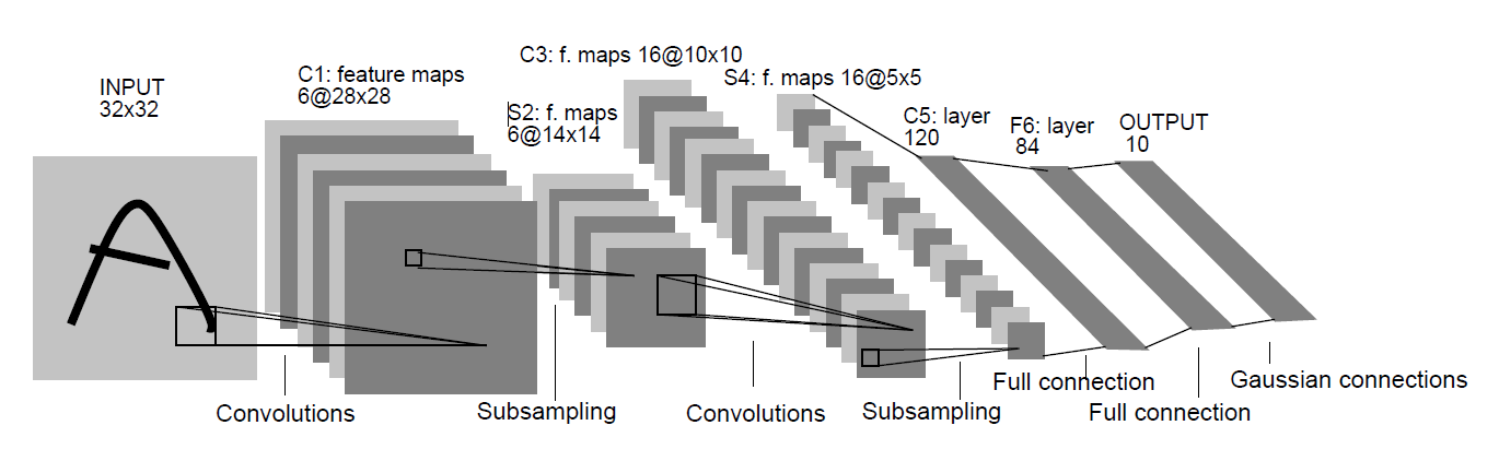
Now, let’s take a better look at how the layers have been stacked up for the model.

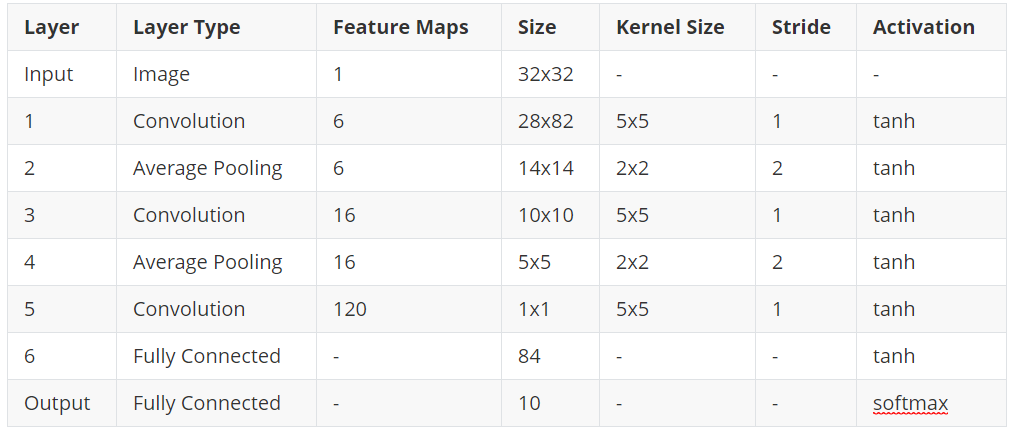
LeNet-5 contains 8 layers in total including the input and output layers. The input is an image of size 32×32. The original MNIST images are 28×28 in size, but for the input layer, they are zero padded to 32×32. Now, there is a very relevant explanation for this. Increasing the size of the input image lets the network recognize the stroke endpoints and corners of the images better.

Then we have the first convolutional layer of size 28×28. The kernel size is 5×5 with tanh activation function. After that, the average pooling layer is present with a kernel size of 2×2 and same tanh activation function. What this layer actually does is that it reduces the size of the previous convolutional layer into half. The layer before it was 28×28, but then, the pooling layer reduces it to 14×14. The same principle follows for two more layers. Before the two fully connected layers we have a convolutional layer with 120 feature maps and size 1×1. Here, the kernel size and activation functions are 5×5 and tanh respectively.

The last two layers are fully connected dense layers. The first fully connected layer has 84 units with tanh activation function. Now, the last layer has 10 units which correspond to each of the 10 digits (from 0 to 9) for the MNIST data set. Here, the activation function is softmax which is very common in many of the output layers in other networks as well, especially for classification purposes.

LeNet-5 in Keras

In this section, we will be using Keras to build our own LeNet-5 model and see how it performs on the MNIST digit data set.

This is going to be a very simple approach with some minor difference. Instead of 32×32 size images, we will be using the default size of 28×28 MNIST images. Also, to replicate the training procedure, we will be using the SGD (Stochastic Gradient Descent) optimizer. So, let’s start.

Import the Required Modules

Let’s import the required packages first. As we will be using tf.keras to build the model, so we do not have to import the standalone Keras packages here.

import matplotlib.pyplot as plt
import tensorflow as tf
import numpy as np

Load and Prepare the Data

Here, we will be loading the MNIST data. We will reshape the data to 4D tensors with channels last input format. We will convert the data into float32 and normalize the pixels as well so that they fall in the range [0.0, 255.0]. Finally, we will one-hot encode the labels which will range from 0 to 9.

mnist = tf.keras.datasets.mnist
(x_train, y_train), (x_test, y_test) = mnist.load_data()

rows, cols = 28, 28

x_train = x_train.reshape(x_train.shape[0], rows, cols, 1)
x_test = x_test.reshape(x_test.shape[0], rows, cols, 1)

input_shape = (rows, cols, 1)

# convert to float and normalize
x_train = x_train.astype('float32')
x_test = x_test.astype('float32')
x_train = x_train / 255.0
x_test = x_test / 255.0

# one-hot encode the labels
y_train = tf.keras.utils.to_categorical(y_train, 10)
y_test = tf.keras.utils.to_categorical(y_test, 10)

Build the Model

In this part, we will define the model inside the build_lenet() function. It will take the input_shape as the parameter. As discussed earlier, we will use the SGD optimizer and the loss is going to be categorical_crossentropy.

def build_lenet(input_shape):
  # sequentail API
  model = tf.keras.Sequential()
  # convolutional layer 1
  model.add(tf.keras.layers.Conv2D(filters=6, 
                                   kernel_size=(5, 5), 
                                   strides=(1, 1),
                                   activation='tanh', 
                                   input_shape=input_shape))
  # average pooling layer 1
  model.add(tf.keras.layers.AveragePooling2D(pool_size=(2, 2), 
                                             strides=(2, 2)))
  # convolutional layer 2
  model.add(tf.keras.layers.Conv2D(filters=16, 
                                   kernel_size=(5, 5), 
                                   strides=(1, 1), 
                                   activation='tanh'))
  # average pooling layer 2 
  model.add(tf.keras.layers.AveragePooling2D(pool_size=(2, 2), 
                                             strides=(2, 2)))
  model.add(tf.keras.layers.Flatten())
  # fully connected
  model.add(tf.keras.layers.Dense(units=120, 
                                   activation='tanh'))
  model.add(tf.keras.layers.Flatten())
  # fully connected
  model.add(tf.keras.layers.Dense(units=84, activation='tanh'))
  # output layer
  model.add(tf.keras.layers.Dense(units=10, activation='softmax'))
  
  model.compile(loss='categorical_crossentropy', 
              optimizer=tf.keras.optimizers.SGD(lr=0.1, momentum=0.0, decay=0.0), 
              metrics=['accuracy'])
  
  return model

lenet = build_lenet(input_shape)

Train the Model

# number of epochs 
epochs = 10
# train the model
history = lenet.fit(x_train, y_train,
                           epochs=epochs, 
                           batch_size=128,
                           verbose=1)

We will train the model for 10 epochs. By the end of training, you should be getting above 98% accuracy.

Test the Model

Let’s test the model on the 10000 test samples.

loss, acc = lenet.evaluate(x_test, y_test)
print('ACCURACY: ', acc)

10000/10000 [==============================] - 1s 62us/sample - loss: 0.0424 - acc: 0.9857 
ACCURACY:  0.9857

Even with not a very deep network, we are getting over 98% test accuracy. You can try to achieve even higher accuracy by augmenting the images while training so that the network will get to see many more images.

Accuracy and Loss Plots

Finally, let’s plot for accuracy and loss.

num_epochs = np.arange(0, 10)
plt.figure(dpi=200)
plt.style.use('ggplot')
plt.plot(num_epochs, history.history['loss'], label='train_loss', c='red')
plt.plot(num_epochs, history.history['accuracy'], label='train_acc', c='green')
plt.title('Training Loss and Accuracy')
plt.xlabel('Epoch')
plt.ylabel('Loss/Accuracy')
plt.legend()
plt.savefig('plot.png')

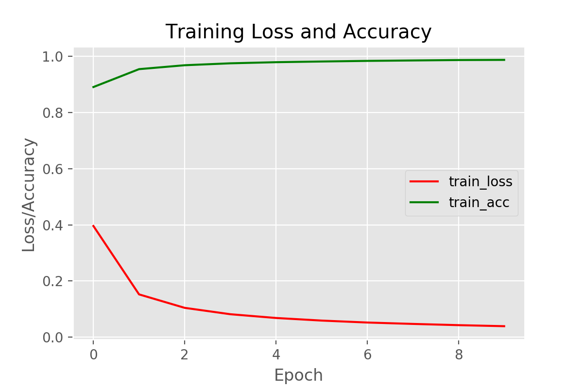
As our model is giving good results, so we see nothing out of context here.

Further Reading

If you want to learn more about the LeNet-5 model, then be sure take a look at the following.
1. LeNet-5 original publication.
2. Yann LeCun’s LeNet-5 demo.

Conclusion

If you liked this article then comment, share and give a thumbs up. If you have any questions or suggestions, just Contact me here. Be sure to subscribe to the website for more content. Follow me on Twitter, LinkedIn, and Facebook to get regular updates.