

In this article, we will go through image classification using deep learning. Image classification is a sub-field of computer vision. There have been a lot of advances in deep learning using neural networks. And because of that computer vision has seen many applications and advances in recent years.
Image classification, image recognition, object detection and localization, and image segmentation are some of those impacted areas.
As computer vision is a very vast field, image classification is just the perfect place to start learning deep learning using neural networks. We will try to cover as much of basic grounds as possible to get you up and running and make you comfortable in this topic.
Overview
The following is a brief overview of what we will be covering in this article:
- A brief about deep learning and neural networks.
- Using Dense Neural Network Layers for image classification.
- Using Convolutional Neural Networks for image classification.
Basically, we will cover two neural network deep learning methods to carry out image classification. This will help you better understand the underlying architectural details in neural networks and how they work.
We will use the Keras library in this tutorial which is very convenient and easy to use.
The Dataset
For the dataset, we will use the Fashion MNIST dataset which is very beginner-friendly. You can visit the GitHub repository here. The dataset contains 60000 training examples and 10000 test examples. Each example is a 28×28 grayscale image.
As we will be using Keras, we can directly download the dataset from the Keras library.
The fashion items in the dataset belong to the following categories.
| Label | Class |
| 0 1 2 3 4 5 6 7 8 9 | T-shirt/top Trouser Pullover Dress Coat Sandal Shirt Sneaker Bag Ankle boot |
You can see that each of the fashion item has a corresponding label from 0 to 9.
Installing Keras and TensorFlow
Before moving further, if you need to install Keras library, then execute the following command in your terminal:
pip install keras
Keras is a high level API and we will be using TensorFlow as the backend. To install TensorFlow, execute the following command:
pip install tensorflow
If your system is having an NVidia GPU, then you can also install the GPU version of TensorFlow using the following command:
pip install tensorflow-gpu
Note: A GPU is not strictly necessary for this tutorial. But training will be faster when using
Deep Learning and Neural Networks
In the past, traditional machine learning techniques have been used for image classification. But neural networks, and mainly Convolutional Neural Networks (thanks to Yann LeCun) totally changed how we deal with computer vision and deep learning today.
In this tutorial, we will be using two different types of layers for image classification. First, we will use the DenseConv2D
Now, you are all set to follow along with the code. If you want, you can type along as you follow.
Load the Libraries
First, we will load all the required libraries and modules.
import numpy as np
import keras
import matplotlib.pyplot as plt

from keras.layers import Dense, Flatten, Conv2D, MaxPooling2D
from keras import Sequential
from keras.datasets import fashion_mnist
Load and Prepare the Data
Now, as we can download and load the Fashion MNIST data from the Keras library.
(x_train, y_train), (x_test, y_test) = fashion_mnist.load_data()
print(x_train.shape)
print(x_test.shape)
print(y_train.shape)
print(y_test.shape)
We have the following output after executing the above code block.
(60000, 28, 28)
(10000, 28, 28)
(60000,)
(10000,)
In x_train, we have 60000 examples with the pixel values of images arranged in a 28×28 matrix. And for y_train, there are 60000 labels ranging from 0 to 9. Similarly for x_test and y_test, which contain 10000 examples and corresponding labels respectively.
The pixel values of the images range from 0.0 to 255.0 and they are all uint8float64
x_train, x_test = (x_train / 255.0).astype('float'), (x_test / 255.0).astype('float')
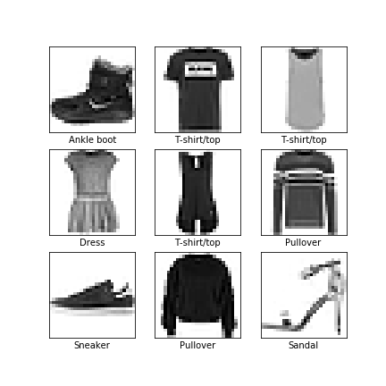
Visualize the Images
It will be a lot easier to analyze the data if we visualize the images in the dataset. First, let’s create a list containing all the fashion item names. This will help us to apply labels to the images in the code.
names = ['T-shirt/top', 'Trouser', 'Pullover', 'Dress', 'Coat', 'Sandal',
        'Shirt', 'Sneaker', 'Bag', 'Ankle boot']
The following block of code generates a plot of the first 9 images in the dataset along with their corresponding names.
plt.figure(figsize=(6, 6))
for i in range(9):
    plt.subplot(3, 3, i+1)
    plt.xticks([])
    plt.yticks([])
    plt.grid(False)
    plt.xlabel(names[y_train[i]])
    plt.imshow(x_train[i], cmap='binary')

plt.savefig('fashion-plot.png')
plt.show()
If you have worked with MNIST handwritten digits before, then you can find a some similarity here. Still, it is a good change and provides just enough complexity to tackle a new type of problem.
Image Classification using Dense Layers
In this section, we will Dense()Sequential()
Build the Mo del
Let’s start by stacking up the layers to build our model.
model_dense = keras.Sequential()
model_dense.add(Flatten(input_shape=(28, 28)))
model_dense.add(Dense(16, activation='relu'))
model_dense.add(Dense(32, activation='relu'))
model_dense.add(Dense(64, activation='relu'))
model_dense.add(Dense(128, activation='relu'))
model_dense.add(Dense(256, activation='relu'))
model_dense.add(Dense(10, activation='softmax'))
Here is a brief analysis of the above code.
First, we initialize the Keras Sequential() model. Then, we use Flatten() which takes input_shape(28, 28) as a parameter. We have observed before that the pixels values are 28×28 matrices. After using Flatten(), the shape changes to (784,). This type of dimension is ideal input for Dense() layers.
After that, we have a Dense() layer with 16 units as the output dimension and relu activation function. We repeat the stacking of such Dense() layers with relu 4 more times till 256 units as the output dimension.
The last Dense() layer has 10 units and softmax activation. We use 10 units as the output can be any one of the class labels from 0 to 9.
We can also print a summary of our model which will give us the parameter details.
print(model_dense.summary())
Model: "sequential_1"
_________________________________________________________________
Layer (type)                 Output Shape              Param #
=================================================================
flatten_1 (Flatten)          (None, 784)               0
_________________________________________________________________
dense_1 (Dense)              (None, 16)                12560
_________________________________________________________________
dense_2 (Dense)              (None, 32)                544
_________________________________________________________________
dense_3 (Dense)              (None, 64)                2112
_________________________________________________________________
dense_4 (Dense)              (None, 128)               8320
_________________________________________________________________
dense_5 (Dense)              (None, 256)               33024
_________________________________________________________________
dense_6 (Dense)              (None, 10)                2570
=================================================================
Total params: 59,130
Trainable params: 59,130
Non-trainable params: 0
_________________________________________________________________
None
In the next section, we are going to compile and train the model
Compile and Train the Model
For compiling the model, we will use adam optimizer and sparse_categorical_crossentropy as the loss. We will monitor the accuracy metric while training.
model_dense.compile(optimizer='adam',
              loss='sparse_categorical_crossentropy',
              metrics=['accuracy'])
Now, we are all set to fit our model. The next snippet of code handles the training of the model.
history = model_dense.fit(x_train, y_train,
                    epochs=10)
Epoch 9/10
60000/60000 [==============================] - 7s 122us/step - loss: 0.3135 - acc: 0.8832
Epoch 10/10
60000/60000 [==============================] - 8s 134us/step - loss: 0.3076 - acc: 0.8853
By the end of the 10\(^{th}\) epoch, we are getting around 88% accuracy.
In the above code, history will store training accuracy and loss values for all epochs, which is 10 in our case. To access the training accuracy and loss values, we can use the following code.
acc = history.history['acc']
loss = history.history['loss']
Using the above data we can plot our training accuracy and loss graphs using matplotlib. That will give us a better insight into our results.
Accuracy and Loss Plots
num_epochs = np.arange(0, 10)
plt.plot(num_epochs, loss, label='train_loss', c='red')
plt.plot(num_epochs, acc, label='train_acc', c='green')

plt.title('Training Loss and Accuracy using Dense Layers')
plt.xlabel('Epoch')
plt.ylabel('Loss/Accuracy')
plt.legend()
plt.savefig('plot1.png')
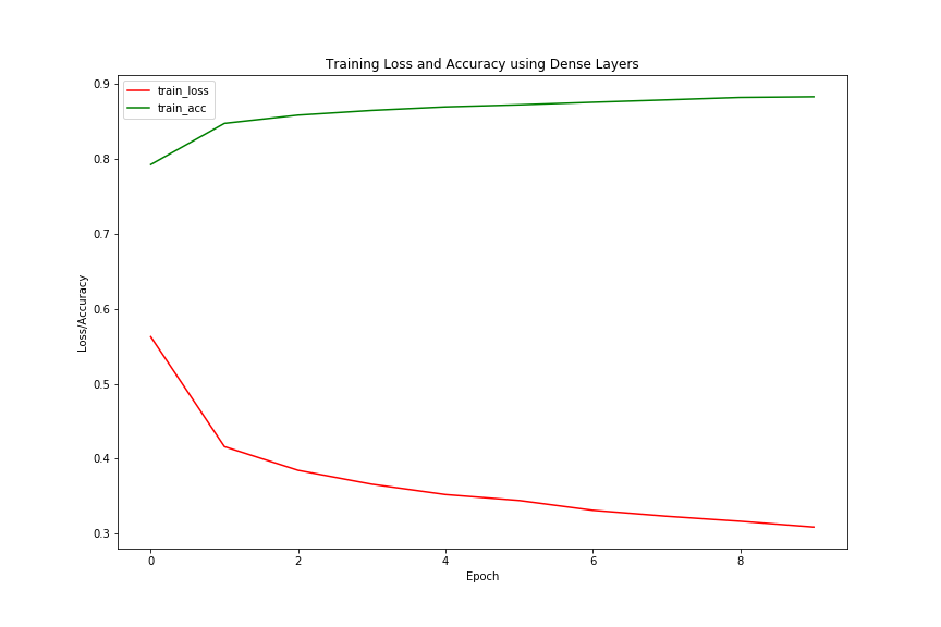
We can see that the loss is decreasing with the increase in the number of epochs and the accuracy is increasing. This is a good sign and shows that our model is working as expected. But what about testing our model on unseen data? After all, we want to see how well our model performs during the test case scenario. For that, we can use evaluate() and get the loss and accuracy scores during testing.
prediction_scores = model_dense.evaluate(x_test, y_test)
print('Accuracy: ', prediction_scores[1]*100)
print('Loss: ', prediction_scores[0])
prediction_scores is a list and it stores two values, the first one is the test loss and the second one is the test accuracy. We can access those values using list indices as we normally do. The above code snippet will output the following:
10000/10000 [==============================] - 1s 51us/step
Accuracy:  87.1
Loss:  0.3684681357383728
We have a test accuracy of 87.1%. We can obviously do better. In the next section, we will use Convolutional Neural Networks and try to increase our test accuracy.
Image Classification using CNN
We have seen how Dense() layers work in Keras. Now we will train on the same dataset but using Conv2D(), which is the Keras implementation of CNN.
CNNs are specially used for computer-vision based deep learning tasks and they work better than other types of architectures for image-based operations.
While using Dense() layers we had to flatten the input. But CNNs take input in a bit different manner. The input shape to a CNN must be of the form (width, height, channel). width and height are common to any 2D image. But what about the channel ?
Well, the channel can be either 1 or 3. If the channel is 1, then it shows that it is a grayscale image. In the grayscale image, each pixel is a different intensity of the color gray.
When the channel is 3, then it shows that it is a colored image composed of three colors, red, green, blue.
In our case, all the images are grayscale images and therefore, the channel is going to be 1. Now, let’s reshape our training and testing data to the ideal input shape for CNN.
# reshape the inputs
x_train = x_train.reshape(x_train.shape[0], x_train.shape[1], x_train.shape[1], 1)
x_test = x_test.reshape(x_test.shape[0], x_test.shape[1], x_test.shape[1], 1)
Now, as we are done with reshaping our data, we can move on to build our model using Sequential().
Build the CNN Model
model_cnn = Sequential()
model_cnn.add(Conv2D(32, input_shape=(28, 28, 1), kernel_size=(3, 3), strides=(2, 2), padding='same', activation='relu'))
model_cnn.add(Conv2D(64, kernel_size=(3, 3), strides=(2, 2), padding='same', activation='relu'))
model_cnn.add(MaxPooling2D(2, 2))
model_cnn.add(Conv2D(128, kernel_size=(3, 3), strides=(2, 2), padding='same', activation='relu'))
model_cnn.add(MaxPooling2D(2, 2))
model_cnn.add(Conv2D(256, kernel_size=(3, 3), strides=(2, 2), padding='same', activation='relu'))
model_cnn.add(Flatten())
model_cnn.add(Dense(10, activation='softmax'))
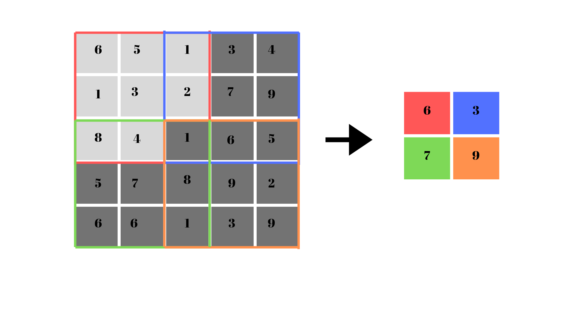
The first layer is a Conv2D() with 32 output dimensionality. The input_shape is (28, 28, 1) as we have discussed above. We can see three new parameters here, they are, kernel_size, strides and padding. Let’s see what each of them does.
kernel_size: this specifies the size of the 2D convolution window in the form of height and width. We have given the window size to be 3×3. strides: we use strides to specify how many rows and columns we skip between each convolution.padding: this is a string which can be either valid or same. In our case, we have used padding='same'.
The following image shows 3×3 kernel size with 2×2 strides.
Next, MaxPooling2D is used to downsample the representations where we have given a pool_size of 2×2 as input. This helps to reduce overfitting and also reduces the number of parameters resulting in faster convergence.
Finally, we flatten the inputs and use a Dense() layer with 10 units for each of the 10 labels.
Compile and Train the Model
The compiling and training part of the model is going to be similar to what we have seen earlier. We will use the same parameters for compiling as in the case of Dense() layer training.
model_cnn.compile(optimizer='adam',
              loss='sparse_categorical_crossentropy',
              metrics=['accuracy'])
history = model_cnn.fit(x_train, y_train,
                    epochs=10)
Epoch 9/10
60000/60000 [==============================] - 8s 136us/step - loss: 0.1686 - acc: 0.9364
Epoch 10/10
60000/60000 [==============================] - 8s 138us/step - loss: 0.1539 - acc: 0.9421
By the end of 10 epochs, we have around 94% training accuracy which is much higher than in the case of Dense() layers.
Accuracy and Loss Plots
acc = history.history['acc']
loss = history.history['loss']

num_epochs = np.arange(0, 10)
plt.figure(figsize=(12, 8))
plt.plot(num_epochs, loss, label='train_loss', c='red')
plt.plot(num_epochs, acc, label='train_acc', c='green')
plt.title('Training Loss and Accuracy using CNN')
plt.xlabel('Epoch')
plt.ylabel('Loss/Accuracy')
plt.legend()
plt.savefig('plot2.png')
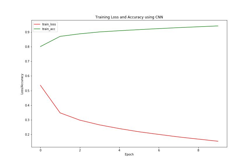
We have more than 90% accuracy during training, but let’s see the test accuracy now.
prediction_scores = model_cnn.evaluate(x_test, y_test)
print('Accuracy: ', prediction_scores[1]*100)
print('Loss: ', prediction_scores[0])
10000/10000 [==============================] - 1s 61us/step
Accuracy:  90.7
Loss:  0.3014533164203167
The test accuracy dopped by a huge margin. Maybe we need more training epochs or maybe a better model architecture to get better accuracy. You should surely play around some more trying to improve the accuracy. You can also post your findings in the comment section.
More Materials to Get Deeper
Deep Learning and Machine Learning Books, Papers and Articles:
- 1. Hands-On Machine Learning with Scikit-Learn, Keras, and TensorFlow, by Aurélien Géron. (Chapters on Deep Learning and CNN)
- 2. LeNet, Yann LeCun
- 3. Convolutional Neural Network Architectures
Summary and Conclusion
In this article, you learned how to carry out image classification using different deep learning architectures. I hope that you liked this article. Subscribe to the website to get more timely articles.
You can also follow me on Twitter and LinkedIn to get notifications about future articles.
