Introduction to XGBoost in Python

XGBoost is a machine learning library that uses gradient boosting under the hood. As XGBoost uses gradient boosting algorithms, therefore, it is both fast and accurate at the same time. It is very efficient at handling huge datasets often having millions of instances. For this reason, XGBoost has become very popular in data science platforms like Kaggle. This article covers an introduction to XGBoost.

In this article, you will be learning:
1. A brief about gradient boosting in machine learning.
2. Introduction and installation of XGBoost.
3. Using XGBoost to classify wine customers. We will Wine Customer Segmentation Kaggle dataset.

Gradient Boosting in Machine Learning

Gradient Boosting is a technique which can be used to build very powerful predictive models, for both classification and regression problems. In gradient boosting we try to convert weak learners into strong learners.

Gradient boosting tries to build an ensemble of learners, mainly decision trees. Decision trees are powerful learning algorithms in themselves. Therefore, an ensemble of decision trees as weak learners makes gradient boosting even more powerful.

Like many machine learning algorithms, gradient boosting also follows the principles of minimizing a suitable cost function using an optimization algorithm.

Least square is one of the most common cost functions used in gradient boosting. We can take the example of Mean Square Error (MSE) as a cost function which we need to reduce. In general, MSE can be defined as,

$$
\frac{1}{n}\sum(\hat{y}-y)^2
$$

In the above formula, \(n\) is the number of examples, \(\hat{y}\) is the predicted output and \(y\) is the actual output.

Introduction to XGBoost

XGBoost is short for Extreme Gradient Boosting. It is a machine learning library which implements gradient boosting in a more optimized way. This makes XGBoost really fast and accurate as well.

XGBoost has gained a lot of popularity in recent years. This is because it can handle huge datasets, even having millions of examples. On data science platforms like Kaggle, XGBoost has been used numerous times to win competitions. This shows how fast and reliable this library is.

Even in the official documentation is says that,

The same code runs on major distributed environment (Hadoop, SGE, MPI) and can solve problems beyond billions of examples.

– XGBoost Documentation

We know how difficult it is in data science to build a model for datasets spanning over millions of examples, let alone billions. For this reason, it can be very useful to learn to use the XGBoost library. Further in the article, we will be building a very simple classifier to get you started with XGBoost.

Installing XGBoost

Installing XGboost is very easy and we can do this using pip command.

Type the following command in your terminal to install XGBoost.

pip install xgboost

There is also GPU support when using XGBoost but in this article, we will use simple XGBoost. If you want to get started with GPU, then consider following the documentation.

About the Dataset

We are using the Wine Customer Segmentation from Kaggle. This dataset is very small and does not showcase the real power of XGBoost. But is a very good dataset for starting out with XGBoost. This will ensure that you understand the usage of XGBoost library properly.

The dataset contains various properties of wine along the feature columns. We need to predict the Customer_Segment column which classifies the wine to a specific segment of customers. We will explore the dataset more as we move along with the coding part.

Using XGBoost on the Wine Segmentation Dataset

Note:It will be better if you follow along with Jupyter Notebook, but you can use any IDE of your choice as well.

First, let’s import all the libraries that we will be needing.

import pandas as pd
import numpy as np
import xgboost
import seaborn as sns
import matplotlib.pyplot as plt

from sklearn.model_selection import train_test_split
from sklearn.metrics import accuracy_score
from sklearn.preprocessing import StandardScaler

np.random.seed(42)

We have imported XGBoost and all other required libraries.

Read and Analyze the Data

In this section, we will read the CSV file, analyze the data and carry out the necessary preprocessing steps.

data = pd.read_csv('Wine.csv')

The following is the structure of the data frame that we have stores in data.

 Alcohol  Malic_Acid   Ash  ...  OD280  Proline  Customer_Segment
0    14.23        1.71  2.43  ...   3.92     1065                 1
1    13.20        1.78  2.14  ...   3.40     1050                 1
2    13.16        2.36  2.67  ...   3.17     1185                 1
3    14.37        1.95  2.50  ...   3.45     1480                 1
4    13.24        2.59  2.87  ...   2.93      735                 1

[5 rows x 14 columns]

We should also take a look at all the columns that are in the dataset.

print(data.columns)

Index(['Alcohol', 'Malic_Acid', 'Ash', 'Ash_Alcanity', 'Magnesium',
       'Total_Phenols', 'Flavanoids', 'Nonflavanoid_Phenols',
       'Proanthocyanins', 'Color_Intensity', 'Hue', 'OD280', 'Proline',
       'Customer_Segment'],
      dtype='object')

Now, let’s check the datatypes of the features. We can ensure whether or not there are any categorical columns that we need to take care of.

# check for data type
print(data.dtypes)

Alcohol                 float64
Malic_Acid              float64
Ash                     float64
Ash_Alcanity            float64
Magnesium                 int64
Total_Phenols           float64
Flavanoids              float64
Nonflavanoid_Phenols    float64
Proanthocyanins         float64
Color_Intensity         float64
Hue                     float64
OD280                   float64
Proline                   int64
Customer_Segment          int64
dtype: object

All the data are in float64 and int64 format. Later we will be converting all the data to float64 format so that our algorithms can work better.

Next, we can take a look at the number of instances in the dataset and also check for the missing values.

# check the number of instances
print(data.shape)

# check for missing values
print(data.isna().sum())

(178, 14)

Alcohol                 0
Malic_Acid              0
Ash                     0
Ash_Alcanity            0
Magnesium               0
Total_Phenols           0
Flavanoids              0
Nonflavanoid_Phenols    0
Proanthocyanins         0
Color_Intensity         0
Hue                     0
OD280                   0
Proline                 0
Customer_Segment        0
dtype: int64

We can see that there are 178 examples in the dataset and 14 columns. Out of the 14 columns, 13 are feature columns and one of the target column (Customer_Segment) that we need to classify.

Also, we do not have any missing values. So, we do not need to worry about handling missing values and carry on further.

Converting all the numerical values to the same datatype will help the algorithm learn better. So, let’s convert all the features into float64 format.

data = data.astype(np.float)

We need to predict Customer_Segment class. Before moving further into creating our training and testing set, let’s visualize the number of customer segment for each class. It will also be better to get the correlation matrix. After that, we will move into preparing our data for training.

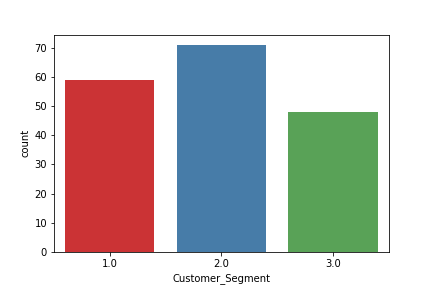
print(data['Customer_Segment'].value_counts())

2.0    71
1.0    59
3.0    48
Name: Customer_Segment, dtype: int64

# customer segment count plot
sns.countplot(data['Customer_Segment'], palette='Set1')
plt.show()
plt.savefig('segment-count.png')

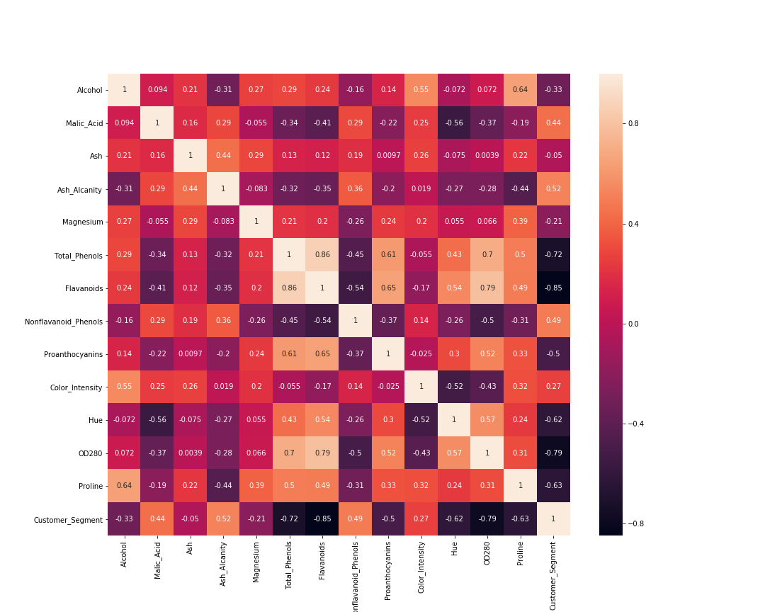
Now, the correlation matrix.

# visaulize the correlation matrix
cor_mat= data[:].corr()
fig=plt.gcf()
fig.set_size_inches(15,12)
sns.heatmap(data=cor_mat, square=True, annot=True, cbar=True)
plt.savefig('corr-matrix.png')
plt.show()

Preparing the Data

In this section, first, we will separate the labels and the features. Next, we will scale the values in our dataset. This will ensure that they all fall within a particular range. It is also helpful for faster gradient descent which in turn results in faster convergence of the algorithm.

# separate the labels and the features
label = data['Customer_Segment']
features_df = data.drop(['Customer_Segment'], axis=1)

# scale the values using StandardScaler()
scaler = StandardScaler()
features = scaler.fit_transform(features_df)

We need to divide the dataset into training and testing set. For that, we will use train_test_split from Scikit-Learn. We will use 80% of the data for training and 20% for testing purposes.

# train-test split
x_train, x_test, y_train, y_test = train_test_split(features, label, train_size=0.8)

Fitting and Prediction

Here, we will initialize the XGBClassifier() and fit our model on the data. We will also carry out predictions on the test set and calculate the accuracy percentage on the predicted classes.

We will use fit() method from XGBoost for training and predict() method to predict the values on the test set.

xgb_clf = xgboost.XGBClassifier()
xgb_clf.fit(x_train, y_train)

# prediction on test set
predictions = xgb_clf.predict(x_test)
# accuracy score
accuracy = accuracy_score(y_test, predictions)
print(np.round(accuracy*100, 2), '%')

Accuracy:  97.22 %

We are getting around 97% accuracy which is a good score. But we should keep in mind that this dataset is really small. XGBoost can handle huge datasets. This tutorial is mainly intended towards getting you started with XGBoost.

Summary and Conclusion

XGBoost classifier has a number of parameters to tune. When we do not specify any values, then it will use default values of the parameters, which it did in the example above. One such parameter is the n_estimators which specifies the number of trees to use. By default, it is 100. Try increasing the number to 500 and see whether there is an improvement.

I hope that gained some valuable insights from this article. Consider subscribing to the website for getting notified about new articles. You can also follow me on Twitter and LinkedIn.