A Guide to XGBoost in Python

Introduction

In this article, we will take a look at the various aspects of the XGBoost library. XGBoost is one of the most reliable machine learning libraries when dealing with huge datasets. In my previous article, I gave a brief introduction about XGBoost on how to use it.

This article will mainly aim towards exploring many of the useful features of XGBoost. When using machine learning libraries, it is not only about building state-of-the-art models. It is also about what types of insights we can gain using the data and tools that we have.

What we will cover in this article:
1. Exploring the simple XGBoost classification.
2. Learning about XGBoost DMatrix.
3. Parameter tuning in XGBoost.
4. XGBoost cross-validation.
5. Feature importances in XGBoost.

Installing XGBoost Library

If you have not installed XGBoost till now, then you can install it easily using the pip command:

pip install xgboost

That’s it. Now you are all set to follow along with this article.

The Dataset

We will use the very popular Titanic dataset from Kaggle. But why this dataset only? This is one of the most famous datasets for beginners in the world of machine learning. Our aim in this article is to learn about the various usages of XGBoost and this is one of the best datasets to do so. This dataset is not very big yet it has enough traction to it that we will be able to explore many aspects when dealing with a machine learning problem.

You can either download the dataset to your local machine or try to follow with the code using Kaggle Kernels.

Note: If you follow along with the code on your local machine, then I suggest that you use Jupyter Notebook, although you can follow any IDE of your choice as well.

So, what do we need to do in this dataset. We are given the train CSV file and the test CSV file. The training file contains the various features of passengers and whether a passenger survived (survival feature) or not (0 or 1). We have to predict the survival key for the test CSV file.

The following is the features table for the dataset.

Variable	Definition	Key
survival	Survival	0 = No, 1 = Yes
pclass	Ticket class	1 = 1st, 2 = 2nd, 3 = 3rd
sex	Sex
Age	Age in years
sibsp	# of siblings / spouses aboard the Titanic
parch	# of parents / children aboard the Titanic
ticket	Ticket number
fare	Passenger fare
cabin	Cabin number
embarked	Port of Embarkation	C = Cherbourg, Q = Queenstown, S = Southampton

Loading, Analyzing and Preprocessing of Data

In this section, we will load the data, analyze it and also preprocess (clean) the data. As our intention is to explore the features of XGBoost, we will go through this phase with a little less explanation. I hope that the code will be self-explanatory.

# necessary imports
import numpy as np
import pandas as pd
import xgboost as xgb
import matplotlib.pyplot as plt

from sklearn.preprocessing import LabelEncoder
from sklearn.metrics import accuracy_score
from sklearn.model_selection import train_test_split

# load the CSV files
data = pd.read_csv('train.csv')

It’s a good idea to check for categorical data types during this stage.

# check categorical
print(data.dtypes)

In the dataset, Name, Sex, Ticket, Cabin, and Embarked are categorical features. And most probably we dot need Name, Ticket, Cabin.

data = data.drop(['Ticket', 'Cabin', 'Name'], axis=1)

# check for missing values
print(data.isna().sum())

Age and Embarked have missing values.

# fill in missing values
data['Age'].fillna(data['Age'].median(), inplace=True)
data['Embarked'].fillna(data['Embarked'].mode()[0], inplace=True)

# label encoding
encoder = LabelEncoder()
for col in ('Sex', 'Embarked'):
    data['Sex'] = encoder.fit_transform(data['Sex'])
    data['Embarked'] = encoder.fit_transform(data['Embarked'])

# separate featues and labels
features = data.drop(['PassengerId', 'Survived'], axis=1)
labels = data['Survived']

# train-test split
x_train, x_val, y_train, y_val = train_test_split(features, labels, train_size=0.85)

We will use 85% data for training and 15% of data for validation.

Using XGBoost DMatrix

We are all set with the preprocessing of data and now we can move ahead to the really important parts of this tutorial.

XGBoost provides a way to convert our training and testing data into DMatrix. DMatrix is an optimized data structure that provides better memory efficiency and training speed. The best part is that converting a dataset into DMatrix is really easy.

The following code converts the training and testing data into DMatrix format.

# convert to DMatrix
d_train = xgb.DMatrix(x_train, y_train)
d_test = xgb.DMatrix(x_val, y_val)

To convert data to DMatrix, we need to give the features of the dataset and then the labels as well.

Setting up Parameters in XGBoost

Now, if you want to train a model on the dataset, then you will need to set some parameters as well. For example, let’s say for the problem we have, we use the following parameters.

In XGBoost, there are numerous parameters. Each is having its own usefulness. But mostly, we can rely on some specific ones for a large set of problems.

params_1 = {
    'booster': 'gbtree',
    'max_depth': 5, 
    'learning_rate': 0.1,
    'sample_type': 'uniform',
    'normalize_type': 'tree',
    'objective': 'binary:hinge',
    'rate_drop': 0.1,
    'n_estimators': 500
}

Okay, let’s go over the parameters briefly:

booster: this specifies the type of booster that XGBoost will use. By default, it is gbtree.
max_depth: it is the maximum depth of the tree. We should be a bit careful while setting this parameter, as a very high value may cause the algorithm to overfit.
learning_rate: this is the learning rate of the algorithm which is set to 0.1. We use this to specify how fast our algorithm will converge to an optimal solution.
sample_type: this is the type of sampling used for dropped trees. This can be either uniform or weighted.
normalize_type: type of normalization algorithm to be used during training. We have used tree.
objective: it is the learning objective for the algorithm. binary: hinge produces classification results, either 0 or 1.
rate_drop: the dropout rate of trees. This has a range from [0.0, 1.0]. We have used 0.1, which tells that 10% of the trees will be dropped.
n_estimators: the number of boosted trees to use while training.

To train on the dataset using a DMatrix, we need to use the XGBoost train() method. The train() method takes two required arguments, the parameters, and the DMatrix. Following is the code for training using DMatrix.

xgb_clf = xgb.train(params_1, d_train)

Using the above model, we can also predict the survival classes on our validation set. We will get the classification results as either 0 or 1. After that, we will calculate the accuracy of our model.

# make prediction
preds = xgb_clf.predict(d_test)

# print accuracy score
print(np.round(accuracy_score(y_val, preds)*100, 2), '%')

83.58 %

k-Fold Cross-Validation in XGBoost

XGBoost also supports cross-validation which we can perform using the cv() method. However, cross-validation is always performed on the whole dataset. The whole data will be used for both, training as well as validation. We will use the nfold parameter to specify the number of folds for the cross-validation.

For k-fold cross-validation, we will need to make a DMatrix consisting of all the training data. Let’s do that first before moving further.

# DMatrix for k-fold cv
dmatrix_data = xgb.DMatrix(features, labels)

Now, we will define the parameters and perform cross-validation for 3 folds.

params = {
    'objective': 'binary:hinge',
    'colsample_bytree': 0.3,
    'learning_rate': 0.1,
    'max_depth': 5,
}

cross_val = xgb.cv(
    params=params,
    dtrain=dmatrix_data, 
    nfold=3,
    num_boost_round=50, 
    early_stopping_rounds=10, 
    metrics='error', 
    as_pandas=True, 
    seed=42)

print(cross_val.head())

You can see some new parameters inside the xgb.cv() method.
num_boost_round: this is the number of boosting iterations that we perform cross-validation for.
early_stopping_rounds: if the validation metric does not improve for the specified rounds (10 in our case), then the cross-validation will stop.
metrics: this is the metric on which cross-validation is evaluated upon. error metric is usually used for binary classification purposes.
as_pandas: we will get the result as a pandas DataFrame.

Printing cross_val will give the results of the cross-validation as a DataFrame.

Visualizing Feature Importance

We can analyze the feature importances very clearly by using the plot_importance() method. This gives the relative importance of all the features in the dataset.

plt.figure(figsize=(16, 12))
xgb.plot_importance(xgb_clf)
plt.show()

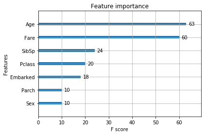
Doing so will give us a very clear idea about our next steps. We can decide which features to include or exclude. Maybe we want to carry out Grid Search or Random Search for getting the optimized parameters. But to see the full effect of XGBoost, you will need much bigger datasets than we have used in this article. This article should act as a guideline for what we can do if we have bigger datasets.

Summary and Conclusion

I hope that this article helped you gain some knowledge about using XGBoost in an efficient way. Do consider subscribing to the website for updates on new articles. Also, leave your thoughts in the comment section about the article.