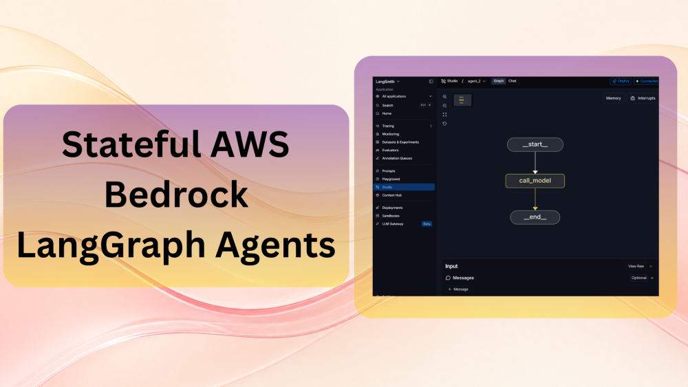
LangChain started as a lightweight framework to connect LLMs with external context and tools. Over the past few years, it has grown to a full-blown ecosystem. With LangGraph for agents and LangSmith for LLM Ops and Observability, we can create an end-to-end agentic system with it. In this article, we will build our first stateful agent using AWS Bedrock, LangGraph, and LangSmith.
When creating agentic systems, we need to define orchestrators, memory layers, session-based memory, and much more. This article will help us understand a few of these concepts to get up and running. Rather than focusing on complex multi-agent systems, we will set up a complete local development workflow, understand how LangGraph organizes projects, and finally build a simple stateful agent with memory.
What will we cover in this article when creating stateful AWS Bedrock LangGraph Agents?
- Setting up the LangGraph development environment and LangSmith
- Creating simple agents with memory
- Calling these agents via LangSmith and LangGraph Studio
Note: We will not cover any complex agents or agent-to-agent interaction. We will simply set up LangGraph Studio & LangSmith and see how to create agents with memory.
Project Directory Structure
Let’s take a look at the directory structure before moving ahead.
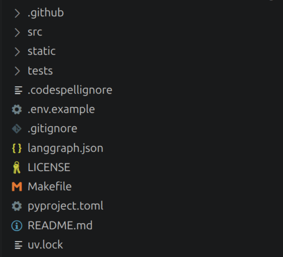
├── src
│   ├── agent_1
│   │   │   ├── graph.cpython-312.pyc
│   │   │   └── graph.cpython-314.pyc
│   │   ├── graph.py
│   │   └── __init__.py
│   └── agent_2
│       │   ├── graph.cpython-312.pyc
│       │   └── graph.cpython-314.pyc
│       ├── graph.py
│       └── __init__.py
├── static
│   └── studio_ui.png
├── tests
│   ├── integration_tests
│   │   │   └── test_graph.cpython-314.pyc
│   │   ├── __init__.py
│   │   └── test_graph.py
│   ├── unit_tests
│   │   ├── __init__.py
│   │   └── test_configuration.py
│   └── conftest.py
├── langgraph.json
├── LICENSE
├── Makefile
├── pyproject.toml
├── README.md
└── uv.lock
We obtain the above directory structure by using an automated setup command, which we will see later in the article.
- The
srcdirectory contains the individual agents that we will customize. After running the setup command, we only see thesrc/agentdirectory. The directory structure shown above has been modified to include multiple custom agents which we will build in this article. - The other file that we need to focus on is
langgraph.json, which contains the information about the individual agents. This is the entry point configuration used by LangGraph Studio. testsdirectory contains the unit and integration tests.
We will take a more detailed look at each component in this article.
The article comes with a compressed version of the above directory. Although we will be building the project from scratch, you can copy and paste the content later to match the workflow that we will cover here.
Download Code
Setting Up LangGraph Studio and LangSmith
In this section, we will complete all the setup steps. I highly recommend creating a new virtual/conda environment with Python 3.12 and following along with the commands.
Setting Up LangGraph and LangSmith
First, we need to install LangGraph with local API server capability.
pip install "langgraph-cli[inmem]"
We install the inmem variant so that LangGraph can run its local development server without requiring Docker. This keeps the setup lightweight and makes it easier to iterate during development.
Second, we need to install langchain-aws to invoke Bedrock models from the LangChain APIs.
pip install langchain-aws==1.6.4
Third, create a new project by executing the following command in your terminal.
langgraph new
It will ask for the directory where you want to set up the project; the current directory is the default choice. It will further ask for the template and the programming language. We choose New LangGraph Project and Python in our case.
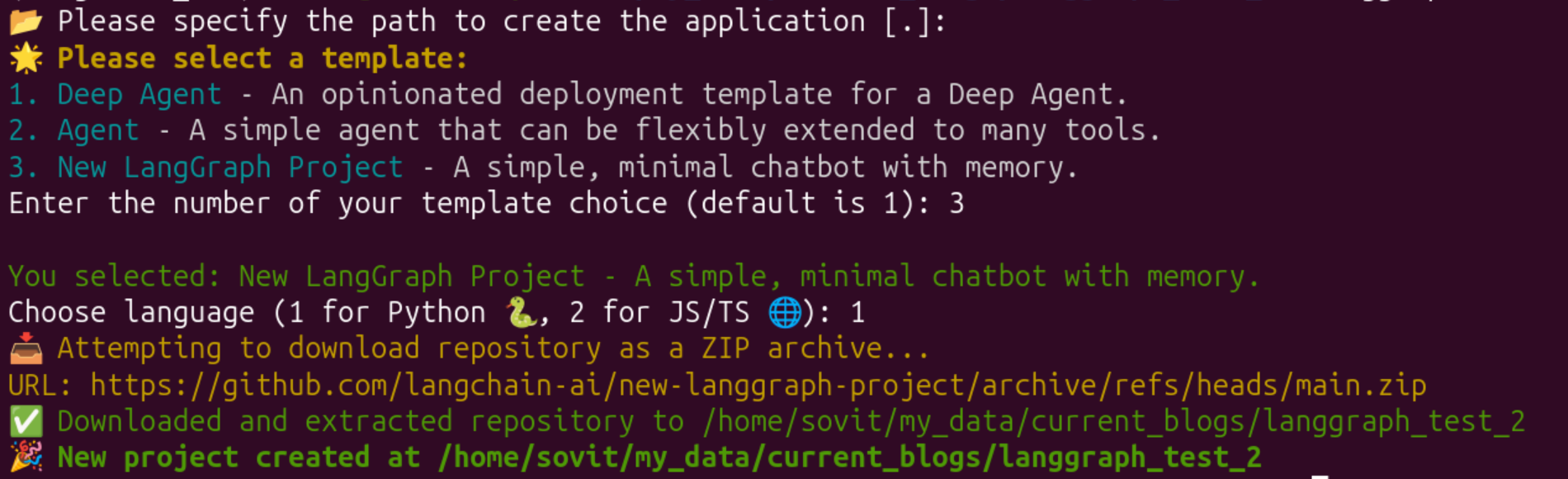
It downloads a templated project that we can use as a starting point and make modifications to according to our requirements. The initial directory structure looks like the following.
One important step before we move into developing agents is creating a LangSmith account with data residency. In this example, we are choosing the AWS US region, which is accessible via the following URL.
Visiting the URL will ask us to create a new account or log in to an existing account. Next, go to Settings => API Keys and create a new API key. Copy the API key, create a .env file in the root directory of the newly created project, and add the following credentials to it.
LANGSMITH_API_KEY=lsv2...
LANGSMITH_ENDPOINT=https://aws.api.smith.langchain.com
The LANGSMITH_ENDPOINT key is important as it tells the application where the data residency is each time we make a call to the agent. Otherwise, the application might ask for logging into the LangSmith dashboard each time we execute a prompt.
Setting Up Bedrock and AWS Credentials
As we are using Amazon Bedrock models in this article, we also need to set up our AWS credentials via the CLI. We will not be covering the creation of an AWS account or setting up IAM roles here.
After setting up a proper IAM role with the necessary permissions for Bedrock, we need to configure the AWS Access Key ID and the AWS Secret Access Key as environment variables. Execute the following command in the terminal to do the same.
aws configure
Important: LangGraph Studio and LangSmith do not automatically read AWS credentials from the project’s .env file. They rely on the credentials configured through the AWS CLI (or standard AWS credential providers). If aws configure has not been run successfully, Bedrock requests will fail even if your .env file contains valid keys.
This is all we need for setting up the initial application. From the next section onward, we will focus on the code.
Building Our First Stateful AWS Bedrock LangGraph Agent
In this section, we will focus on creating our first agent with Bedrock and LangGraph. The code for this lives in the src/agent_1/graph.py file. We can rename the agent_1 directory to anything of our choice, and that will work as the name for that agent.
Note: When we first generate the project template, a default agent with a dummy output is present. We have made modifications to the agent code by adding memory checkpoint capability and using Bedrock as the LLM provider.
The following block shows the entire code.
from dataclasses import dataclass, field
from typing import Any, Dict, Annotated

from langchain_aws import ChatBedrockConverse
from langchain_core.messages import BaseMessage
from langgraph.graph import StateGraph
from langgraph.graph.message import add_messages
from langgraph.runtime import Runtime
from typing_extensions import TypedDict

class Context(TypedDict):
    """Context parameters for the agent.

    Set these when creating assistants OR when invoking the graph.
    See: https://langchain-ai.github.io/langgraph/cloud/how-tos/configuration_cloud/
    """

    my_configurable_param: str

@dataclass
class State:
    """State schema with a message history reducer."""
    messages: Annotated[list[BaseMessage], add_messages] = field(default_factory=list)


async def call_model(state: State, runtime: Runtime[Context]) -> Dict[str, Any]:
    """Process message history using ChatBedrockConverse and return response messages."""
    model = ChatBedrockConverse(
        model="amazon.nova-pro-v1:0"
    )

    # Pass the full message history directly to the model
    response = await model.ainvoke(state.messages)

    # Return the assistant message to be added via the add_messages reducer
    return {"messages": [response]}

# Define the graph
graph = (
    StateGraph(State, context_schema=Context)
    .add_node(call_model)
    .add_edge("__start__", "call_model")
    .compile(name="New Graph")
)
Before jumping into the explanation of the code, let’s understand what is happening in the above code. We know that we have created an agent, and it answers the user’s questions. But what does the data flow look like?
User Message
      │
      ▼
Graph State
      │
      ▼
call_model()
      │
      ▼
Amazon Bedrock
      │
      ▼
Assistant Response
      │
      ▼
State Updated
Unlike a traditional chatbot where we explicitly call the model inside a loop, LangGraph represents the workflow as a graph. Each node performs one task, receives the current state, modifies it, and passes it to the next node.
We can simply think of a single node as a function doing a logical task. Several nodes may be connected by edges that pass on the information after the node has performed the task.
Defining the Agent State
The State class is the only shared state here. It manages the messages list that we use for storing chat turns from both the user and the agent. The add_messages reducer manages the entirety of conversation history storage internally.
Let’s understand with an example.
The User says:
Hello
The State becomes:
[
 HumanMessage(...)
]
Assistant replies:
Hi
The reducer modifies the State to:
[
 HumanMessage(...),
 AIMessage(...)
]
If we do not use the add_messages reducer, the returned value, be it from User or Assistant, replaces the existing messages list, resulting in loss of conversation history. For example:
[
 AIMessage(...)
]
And that’s how the conversation history is stored.
The Model Node
The call_model() function is the only node that we have here. The basic workflow looks like the following:
User State (input)
  ↓
Node (calls Bedrock)
  ↓
Returns (AI response)
As LangGraph merges returned values into the graph state, we always get the response in the form of a dictionary, e.g., {"messages":[response]}. We will understand this more clearly when invoking the agent via LangGraph Studio.
Furthermore, the node never returns the whole message history, as the add_messages is already working in the background to append the responses to the messages list.
The StateGraph
One of the more important components is the StateGraph.
graph = (
    StateGraph(State, context_schema=Context)
    .add_node(call_model)
    .add_edge("__start__", "call_model")
    .compile(name="New Graph")
)
This is a directed graph where the nodes are functions and edges define the information flow. For example, in the above code, call_model is our only node. The add_edge method defines that after the graph execution starts, it will go to call_model. The information is only shared between the __start__ node (which is implicit) and the call_model node (which we have defined). Finally, the compile() method converts the graph definition into an executable application that we can invoke independently. For the above graph, the entire workflow and data lives in these two nodes:
┌───────────┐
│ __start__ │
└─────┬─────┘
      │
      ▼
┌────────────────┐
│  call_model()  │
└────────────────┘
There is another agent that we have defined in src/agent_2/graph.py. However, it is an exact copy of the above agent. The only reason to include that is to understand how to define multiple agents, how to modify the agent JSON file, and how we navigate the studio environment.
Finally, the Context object is used for runtime configuration. We won’t use it in this article, but the template includes it so that configuration values can be passed to the graph during invocation.
Understanding the LangGraph JSON File
Before moving to agent invocation, let’s take a look at the langgraph.json file in the project’s root directory.
{
  "$schema": "https://langgra.ph/schema.json",
  "dependencies": ["."],
  "graphs": {
    "agent_1": "./src/agent_1/graph.py:graph",
    "agent_2": "./src/agent_2/graph.py:graph"
  },
  "env": ".env",
  "image_distro": "wolfi"
}
Every agent that we want LangGraph Studio to discover must be registered under the graphs section. Each entry maps an agent name to a Python object in the format:
path/to/file.py:graph
Here, graph refers to the compiled StateGraph object that we created in graph.py. When LangGraph Studio starts, it reads this file to determine which agents should be loaded.
With this, we are done with all the agent definitions. Next, we will move to starting LangGraph Studio and executing the agent invocation.
Agent Invocation via LangGraph Studio
Execute the following command in the project’s root directory:
langgraph dev
It should automatically open the Studio environment in your default browser, or you can click on the link in the terminal, which is similar to this:
- https://aws.smith.langchain.com/studio/?baseUrl=http://127.0.0.1:2024
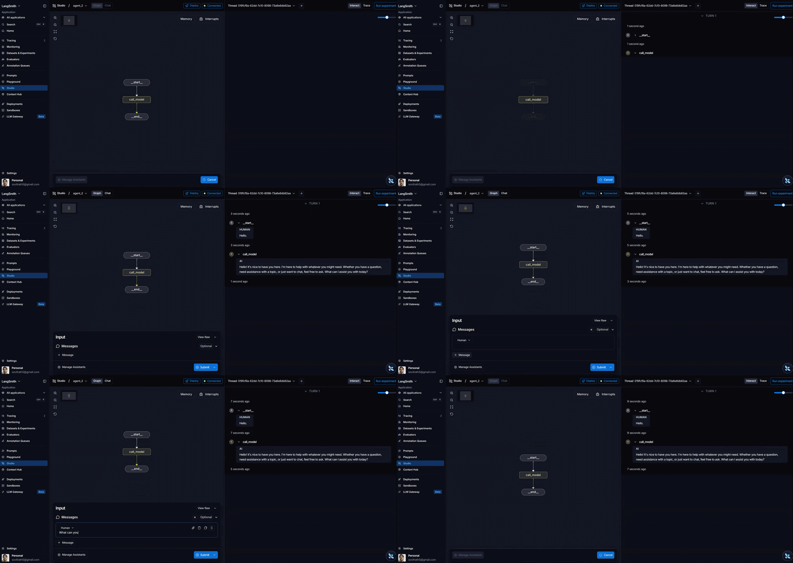
This is how the home screen looks.
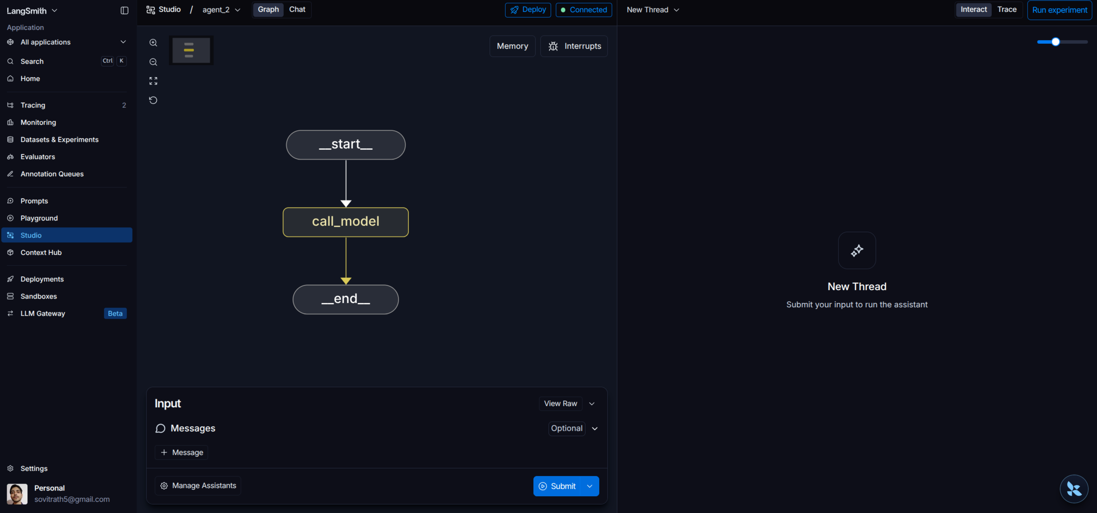
We have the selected agent graph, an input box for a message, and the right tab shows the results from the agent.
The following video shows an end-to-end workflow when the user inputs a message and gets a response from the agent.
We can see that each response is a dictionary from the agent. Whenever we deploy or use these agents in other applications, we can extract the necessary values from the response dictionary and act on them. We can easily capture the streaming response as well.
We can also choose between the agents from the top dropdown if we are testing multiple agents.
Summary and Conclusion
In this article, we covered an introduction to building stateful LangGraph agents with AWS Bedrock. We started with the basic setup, moved to understanding what an agent graph does, and how to invoke them via LangGraph Studio. Although we did not cover how to use these agents in external applications, creating multiple agents with different capabilities, or adding tools for these agents, we will do that in future articles. I hope this article was worth your time.
If you have any questions, thoughts, or suggestions, please leave them in the comment section. I will surely address them.
You can contact me using the Contact section. You can also find me on LinkedIn, and X.