

In this part of the Deep Learning with Keras series, we will learn some of the most useful concepts. We will cover topics like Callbacks in Keras, saving models and restoring models. You will also learn about Tensorboard visualization which is an important part of Keras callbacks and analyzing and training models.
This is the fifth part of the series Introduction to Keras Deep Learning.
Part 1: Getting Started with Keras.
Part 2: Learning about the Keras API.
Part 3: Using Keras Sequential Model.
Part 4: Regression using Neural Network.
Part 5: Using Callbacks and ConvNets.
If you have been following this series, then you must have installed the Anaconda distribution. For saving models, we will use the .h5 format. If you are reading this article directly, then you may want to install a few packages.
Install the Required Packages
Install h5py with pip:
pip install h5py
To install h5py with the conda command:
conda install -c anaconda h5py
Now, to install Tensorboard using the pip command, type the following:
pip install tensorboard
And, if you want to use the conda command to install Tensorboard, then do the following:
conda install -c conda-forge tensorboard
Callbacks in Keras
The Dataset
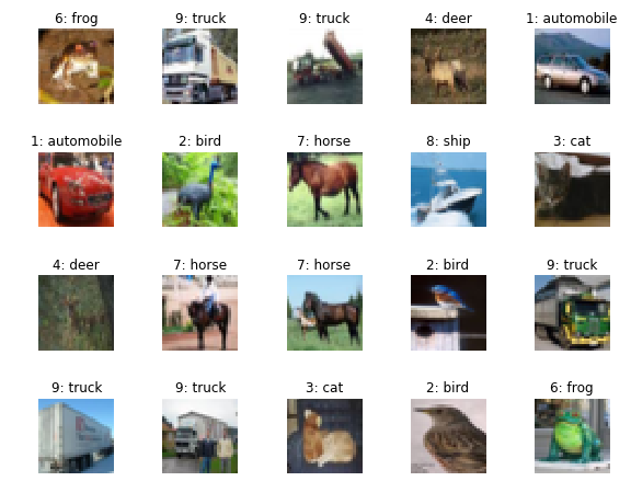
This time, we will use the CIFAR10 dataset to carry out classification. The CIFAR10 dataset contains 60000 labeled images distributed among 10 classes. So, there are 6000 images belonging to each class. The following are the label classes in the dataset:
airplane
automobile
bird
cat
deer
dog
frog
horse
ship
truck
The Neural Network Model
We will be using a convolutional neural network to build the model. More specifically, we will use Conv2D layers instead of Dense. For classifying CIFAR10 images, convolutional neural networks work much better that simple Dense networks.
You can visit one of the previous posts to know more about convolutional neural networks.
Now, we are all set to get into the coding part.
Required Imports
Let’s import all the required packages and modules we will need further into the article.
import numpy as np
import matplotlib.pyplot as plt
import random
import time

from keras.layers import Dense, Flatten, Conv2D, MaxPooling2D, Dropout
from keras.callbacks import EarlyStopping, TensorBoard, ModelCheckpoint
from keras.datasets import cifar10
from keras.models import Sequential, load_model
from keras import optimizers
To keep things simple, we will use Sequential() model to build our network. EarlyStopping will let us stop our training when the observed metric does not improve for a certain number of epochs. And ModelCheckpoint will help us to save the best model during training.
For, reproducibility, let’s generate a random seed.
# for reproducibility
np.random.seed(42)
Download the Dataset
We can download the dataset directly from the Keras library.
(x_train, y_train), (x_test, y_test) = cifar10.load_data()
Data Preparation
This section is pretty important. We will normalize the pixel values by dividing the pixel values by 255.0. This will make the pixel values to fall between 0.0 and 1.0.
Next, we will categorize the train and test labels as well. For example, from the image of the classes above, we know that for the pixel values corresponding to a bird, the label is 2. After we categorize the labels, each of the instances will have 10 values in the label column. But all except one will be zero. The index value corresponding to the label will be 1. So, for a bird, index position 2 will have the value 1.
The following blocks of code carry out the above operations.
# normalize the pixel values
x_train, x_test = x_train / 255.0, x_test / 255.0
# take a look at the labels
y_train = to_categorical(y_train, num_classes=10)
y_test = to_categorical(y_test, num_classes=10)

y_train
[[0. 1. 0. ... 0. 0. 0.]
[1. 0. 0. ... 0. 0. 0.]
[1. 0. 0. ... 0. 0. 0.]
...
Now, looking at the shapes of the training and testing set will give us a good idea about the number of instances in each.
print(x_train.shape)
print(y_train.shape)
print(x_test.shape)
print(y_test.shape)
(50000, 32, 32, 3)
(50000, 10)
(10000, 32, 32, 3)
(10000, 10)
We have 50000 instances for training and 10000 for testing purposes. The images are all 32×32 in size and are colored as well.
Next, we create all the callbacks that we are going to use during the training.
# create the callbacks
NAME = 'cifar10-{}'.format(int(time.time())) # to save different tensorboard logs each time

tensorboard = TensorBoard(log_dir='logs/{}'.format(NAME))

# early stopping
stop = EarlyStopping(monitor='val_loss', mode='min', verbose=1, patience=10)
# define checkpoints
checkpoint = ModelCheckpoint('cifar10_best_model.h5', monitor='val_acc', mode='max', verbose=1, save_best_only=True)
To save different Tensorboard logs each time, we are formatting the name on the basis of time. All the logs will be saved in the logs directory.
For EarlyStopping, we will monitor the validation loss. If the validation loss does not improve for 10 epochs, then the training will stop.
We do not need to save the models after each epoch. Therefore, we are using ModelCheckpoint callback. For this, we will monitor the validation accuracy. This means that we will save the model after an epoch only if the validation accuracy improves in comparison to the previous epochs.
Building the Model
Okay, we will build our neural network model now. As discussed in the beginning, we will use the Keras Sequential() to build the model.
The following is the code for building the model.
# stacking up the layers
model = Sequential()

model.add(Conv2D(32, kernel_size=(3, 3), activation='relu', input_shape=(32, 32, 3)))
model.add(Conv2D(64, kernel_size=(3, 3), activation='relu'))
model.add(MaxPooling2D(pool_size=(2, 2)))
model.add(Dropout(0.25))

model.add(Conv2D(128, kernel_size=(3, 3), activation='relu'))
model.add(MaxPooling2D(pool_size=(2, 2)))
model.add(Conv2D(128, kernel_size=(3, 3), activation='relu'))
model.add(MaxPooling2D(pool_size=(2, 2)))
model.add(Dropout(0.25))

model.add(Flatten())
model.add(Dense(1024, activation='relu'))
model.add(Dropout(0.5))
model.add(Dense(10, activation='softmax'))
For the first layer, we use Conv2D() with 32 dimensions and kernel_size of 3×3. The activation function is ReLU. The input shape is (32, 32, 3), which means that it is a channels last input. Then we have another Conv2D() with 64 dimensions. The MaxPooling2D() has a pool_size of 2×2. This means that it will reduce the output dimensions by half for the next layer. We also use a Dropout() of 0.25 before ending the layer.
The next two layers are composed of Conv2D() and MaxPooling2D() each. The output dimensions for both the Conv2D()s are is 128. Also, we use a Dropout() of 0.25 as well.
Next, we have Flatten() to flatten out the dimensions. After that, we use a Dense() with 1024 units. The final Dropout() before the last Dense() layer is 0.5. Finally, we end the deep neural network with a Dense() layer of 10 units and softmax activation function.
Compile the Keras Model
For compiling the model, we will use Adam optimizer. The loss is going to be categorical_crossentropy and metric will be accuracy.
optimizer = optimizers.Adam()
model.compile(loss='categorical_crossentropy',
              optimizer=optimizer,
              metrics=['accuracy'])
Train the Model
Now, it is time to train the model.
history = model.fit(x_train, y_train,
                    epochs=100,
                    validation_split=0.2,
                    callbacks=[tensorboard, stop, checkpoint])
We train the model for 100 epochs. But as we have also provided the callbacks, there is a very high probability that the training will stop way before reaching 100 epochs. Also, 20% of the data is split for validation purpose.
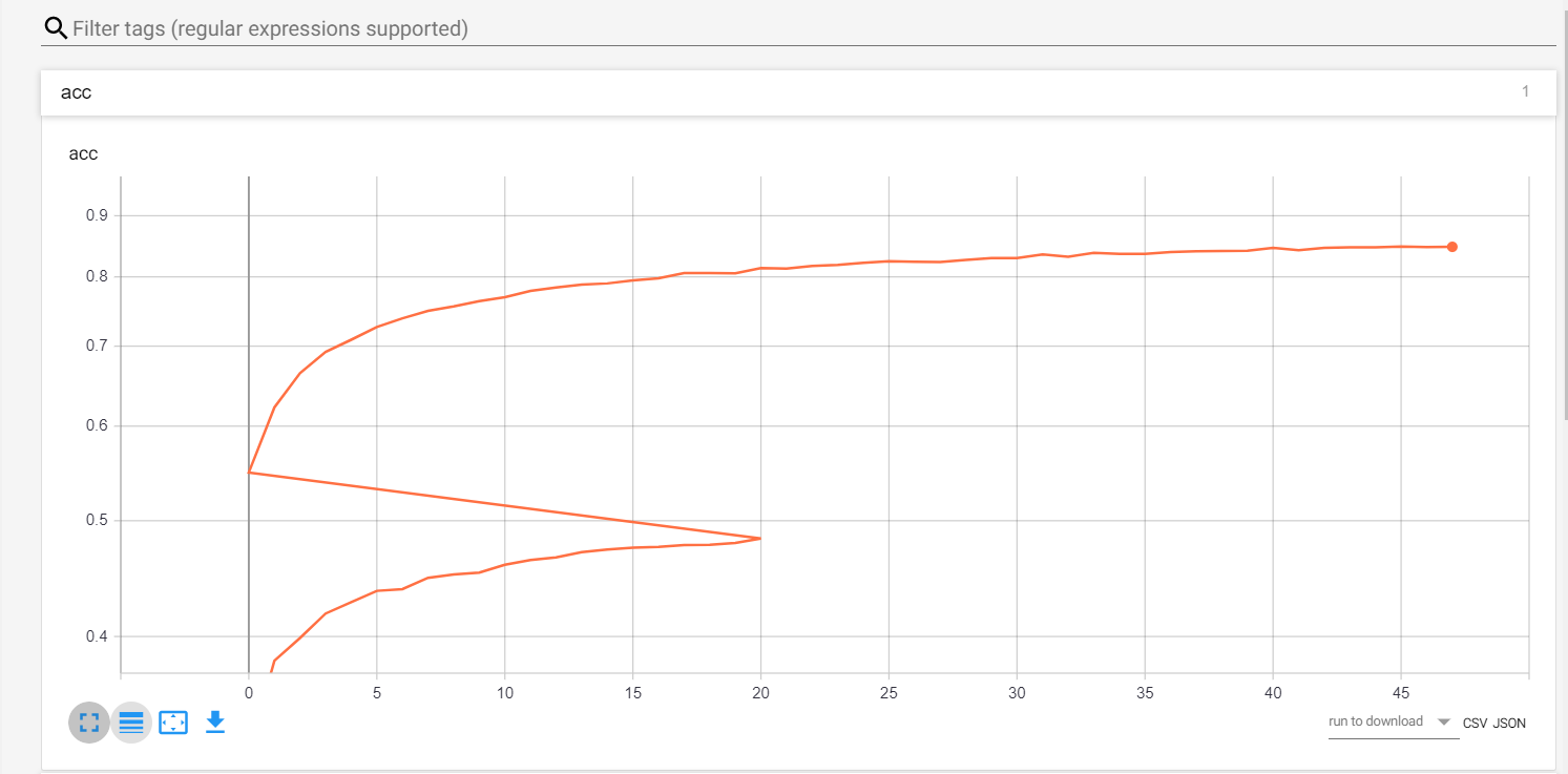
During training, you can use Tensorbaord to monitor the graphs of accuracies and losses. To do so, open up a new terminal and head over to your project directory. Then, type the following command:
tensorboard --logdir=logs/
Next, head over to http://localhost:6006/ in your browser. You should see Tensorboard along with the accuracy and loss plots updating as the training continues. This is a good way to monitor model training when doing large scale projects.
Prediction and Accuracy
Here, we will predict the classes for the test set and also find the accuracy of the model. Before that, let’s load the best model that has been saved.
model = load_model('cifar10_best_model.h5')
preds = model.predict(x_test)

loss, accuracy = model.evaluate(x_test, y_test)
print('LOSS: ', loss)
print('ACCURACY: ', accuracy*100)
LOSS:  0.7353132239341735
ACCURACY:  76.84
The result is not too satisfactory. But you can always try to improve the model by different preprocessing methods. For a start, you should try augmenting the images, so that the model gets to see much more image data than initially provided. If you need a head start with image augmentation, then do consider visiting this article.
Summary and Conclusion
In this article, you learned to train a model using callbacks in Keras. You also learned how to use TensorBoard to monitor the training plots.
If you liked this article, then share this with others. Subscribe to the website to get regular updates directly into your inbox. You can follow me on LinkedIn and Twitter as well.
