Introduction to Deep Learning with Keras (Part 3): Using Keras Sequential Model

In this post, we are going to learn about the Keras Sequential Model and how to use it to build our own deep neural network. If you are following this tutorial series, then this is going to be your first major step in deep learning with Keras. We will be using Keras deep learning to build a classification network.

This is the third part of the series Introduction to Keras Deep Learning.
Part 1: Getting Started with Keras.
Part 2: Learning about the Keras API.
Part 3: Using Keras Sequential Model.

What will You Learn in this Article

• About Keras Sequential Model in detail.
• How to build your own deep neural network?
• Building a Dense Neural Network for classifying Fashion MNIST images.

Before Starting

When starting with deep learning, the most common dataset that people use is the MNIST handwritten digits data set. But we will be using a newer MNIST data set, that is the fashion MNIST images data set. This contains images of different fashion items which are divided into 10 classes.

This data set is very similar to the hand-written digits data set. It contains 60000 training samples and 10000 test samples with each being a greyscale image of size 28×28.

This data set is perfect for starting out with deep learning as it is just slightly more challenging than the hand-written digits data set. If you want you can go take a look at one of the previous articles which take you through the MNIST digit classification first.

Now, let’s get to the coding part.

Necessary Imports

First, we should import all the required packages.

import numpy as np
import matplotlib.pyplot as plt
import keras
import keras.layers

from keras import optimizers
from keras import Sequential
from keras.layers import Dense, Flatten

We will be using Dense() layer to build our neural network. This means that our model will consist of densely connected neural network layers.

Also, Flatten() will help us to flatten the input shape.

Load the Data

The Fashion MNIST data set is already included in the Keras API. That means we can directly load the data by calling datasets module.

fashion_mnist = keras.datasets.fashion_mnist
 
(x_train, y_train), (x_test, y_test) = fashion_mnist.load_data()

The tuples x_train and y_train hold the training data and training labels respectively. Similarly, the test data and labels are stored in x_test and y_test.

Analyzing the Data

The data set contains images of 10 types of fashion items.

Label	Description
0	T-shirt/top
1	Trouser
2	Pullover
3	Dress
4	Coat
5	Sandal
6	Shirt
7	Sneaker
8	Bag
9	Ankle boot

We can make a list of these items which will help us while visualizing the images later.

names = ['T-shirt/top', 'Trouser', 'Pullover', 'Dress', 'Coat', 'Sandal', 
        'Shirt', 'Sneaker', 'Bag', 'Ankle boot']

Now, the data in y_train are labeled as per the table. So, if it is 0, then the item is a T-shirt/top and so on.

print(y_train)

[9 0 0 ... 3 0 5]

Let’s look at all the shapes of the data sets.

print(x_train.shape)
print(y_train.shape)
print(x_test.shape)
print(y_test.shape)

(60000, 28, 28)
(60000,)
(10000, 28, 28) 
(10000,)

So, the train data and labels contain 60000 instances each and test data and labels contain 10000 instances.

Normalizing the Data

When dealing with neural networks, it is always better to normalize the data. After normalization, the data will range from 0.0 to 1.0. We know that the pixel values can be anything between 0.0 and 255.0. Therefore, we can normalize the pixel values by diving them with 255.0.

# scaling the images
x_train, x_test = x_train / 255.0, x_test / 255.0

After scaling the data, the neural network will be able to learn much faster. Neural networks always work better with floating-point values.

Visualizing the Images

Before building our model, let’s visualize some of the images that are available in the data set. This will give us a better idea about what type of images we are dealing with.

plt.figure(figsize=(12, 8))
for i in range(9):
    plt.subplot(330+i+1)
    plt.xticks([])
    plt.yticks([])
    plt.grid(False)
    plt.imshow(x_train[i])
    plt.xlabel(names[y_train[i]])
    
plt.colorbar()
plt.show()

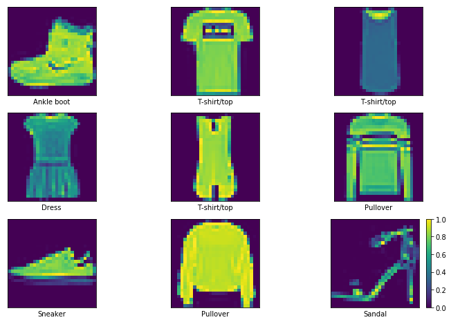
The color bar at the end shows that the pixels are already scaled with the minimum value of 0.0 and the maximum value of 1.0.

Building the Model in Keras

Now, we can proceed to build the model using Keras API. We will use the Sequential() model. The first layer will be a Flatten() that will take the dimensions of the dataset as the input.

Then we will continue with two hidden Dense() layers after that. The first one will have an output dimension of 64 and the second one will have 128 as the output dimension. Both the hidden layers will have the relu activation function.

The last dense layer will have an output dimension of 10. This is because we can get any number between 0 and 1 as the output. This layer will use the softmax activation function.

Let’s get into the code for building the model.

# stacking up the layers
model = keras.Sequential()
model.add(Flatten(input_shape=(28, 28)))
model.add(Dense(64, activation='relu'))
model.add(Dense(128, activation='relu'))
model.add(Dense(10, activation='softmax'))

Compile the Model

The next step is to compile the model.

# compiling the model
optimizer = optimizers.adam()
model.compile(optimizer=optimizer, 
             loss='sparse_categorical_crossentropy',
             metrics=['accuracy'])

Here, we are using the adam() optimizer. We are not passing any custom learning rate or decay parameter. As this is the first classification tutorial in the series, it is better to keep things simple. But if you really want to change the parameters, then take a look at the documentation.

Our model is going to output a single integer for each of the images. Therefore, the loss is sparse_categotical_crossentropy. And we will be monitoring the accuracy metric.

Train the Model

This part is really simple. We just need to use the fit() method to train the model. The input parameters will be x_train and y_train. We will train the model for 10 epochs.

model.fit(x_train, y_train, epochs=10)

Epoch 1/10 60000/60000 [==============================] - 7s 108us/step - loss: 0.5043 - acc: 0.8203 
Epoch 2/10 60000/60000 [==============================] - 5s 90us/step - loss: 0.3753 - acc: 0.8626 ...

By the end of the training, you should be getting around 90% accuracy. But we are more interested in the prediction accuracy, that is how our model performs on unseen data.

Evaluate the Model

accuracy = model.evaluate(x_test, y_test)
print('Accuracy:', accuracy)

10000/10000 [==============================] - 0s 43us/step 
Accuracy: [0.33399120326042175, 0.8824]

We are getting around 0.333 loss and 88% accuracy. This is not very good but not too bad for a start as well. In future posts, we will see how to increase accuracy even further.

Summary and Conclusion

In this tutorial, you learned how to build a simple neural network classifier. You can try and fiddle with the various optimizer parameters and see how it affects the model run time and accuracy. We will get into more details in the upcoming posts.

Subscribe to the website to get the updates right in your inbox. Like and share this post. You can also follow me on Twitter and LinkedIn.