Introduction to Deep Learning with Keras (Part 4): Regression using Keras

In this article, we will be using Keras for regression. In classification, we predict the discrete classes of the instances. But in regression, we will be predicting continuous numeric values. We will use Keras to build our deep neural network in this article.

This is the fourth part of the series Introduction to Keras Deep Learning.
Part 1: Getting Started with Keras.
Part 2: Learning about the Keras API.
Part 3: Using Keras Sequential Model.
Part 4: Regression using Neural Network.

The Dataset

We will use the Auto MPG dataset from UCI Machine Learning Repository. This dataset contains fule consumptions of several vehicles in miles per gallon. So, we need to predict the fuel efficiencies of various vehicles from the data that has been provided.

To download the data, you can follow this link and then download the file auto-mpg.data.

Okay, now we are ready to get into the coding part. You can use your own jupyter notebook or Google colab to follow along.

Import the Libraries

import numpy as np
import pandas as pd
import seaborn as sns
import matplotlib.pyplot as plt
import keras

from keras import Sequential
from keras.layers import Dense
from sklearn.model_selection import train_test_split

Load the Data

Let’s load the data now. As this is not a csv file, we need to use pandas read_table method to read the data.

data = pd.read_table('auto-mpg.data')

Analyze the Data

In the dataset website, you can find under the Attribute Information section, that there are 9 attributes. Those are:
1. mpg: continuous 
2. cylinders: multi-valued discrete 
3. displacement: continuous 
4. horsepower: continuous 
5. weight: continuous 
6. acceleration: continuous 
7. model year: multi-valued discrete 
8. origin: multi-valued discrete 
9. car name: string (unique for each instance)

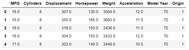
Currently, the data is not in a very readable format.

data.head()

For the above code, you will get the following output.

18.0 8 307.0 130.0 3504. 12.0 70 1chevrolet chevelle malibu
015.0 8 350.0 165.0 3693. 11...buick skylark 320
118.0 8 318.0 150.0 3436. 11...plymouth satellite
216.0 8 304.0 150.0 3433. 12...amc rebel sst
317.0 8 302.0 140.0 3449. 10...ford torino
415.0 8 429.0 198.0 4341. 10...ford galaxie 500

We need to give column names to the dataset and change it to csv readable format. The following block of code will help us do that.

column_names = ['MPG','Cylinders','Displacement','Horsepower','Weight',
                'Acceleration', 'Model Year', 'Origin']
csv_data = pd.read_csv('auto-mpg.data', names=column_names,
                        na_values = "?",
                        comment='\t',
                        sep=" ", 
                        skipinitialspace=True)

dataset = csv_data.copy()
dataset.head()

The above code should give the following output.

Clean the Data

Now, let’s print the data types of the attributes.

print(dataset.dtypes)

MPG             float64 
Cylinders         int64 
Displacement    float64 
Horsepower      float64 
Weight          float64 
Acceleration    float64 
Model Year        int64 
Origin            int64 
dtype: object

Although all the data above are listed as either float64 and int64, we know that Cylinders, Model Year, and Origin are actually discrete values. And the Origin attribute can actually introduce some bias into the network if we do not one-hot encode it.

We should first see how many categories Origin has.

print(dataset.Origin.value_counts())

1 249
3 79
2 70
Name: Origin, dtype: int64

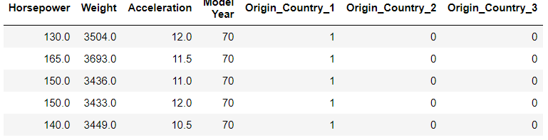
The attribute has 3 categories. It is always better to create a copy of the dataset before creating dummy variables. So, the following code can help us to one-hot encode the attribute.

dataset_copy = dataset.copy()
dataset_copy = pd.get_dummies(dataset_copy, columns=['Origin'], 
                              prefix=['Origin_Country'])
dataset_copy.head()

Next, we should try to clean the data of any missing values.

print(dataset_copy.isna().sum())

MPG                 0 
Cylinders           0 
Displacement        0 
Horsepower          6 
Weight              0 
Acceleration        0 
Model Year          0 
Origin_Country_1    0 
Origin_Country_2    0 
Origin_Country_3    0 
dtype: int64

Horsepower attribute has 6 missing values. We can drop those rows as dropping 6 rows from the dataset will not affect the training of the network much.

# drop the missing value instances
dataset_copy = dataset_copy.dropna()

Train and Test Set

We are ready to divide the data into train and test set. We will be using 80% of the data for training and 20% for testing.

labels = dataset_copy['MPG']
train_data = dataset_copy.drop(['MPG'], axis=1)

x_train, x_test, y_train, y_test = train_test_split(train_data, labels,
                                                    test_size=0.2)

Normalize the Data

Normalization of the data is a very important step and is done in almost any machine learning project. The range of the values in the dataset vary greatly. This can adversely affect the training of the neural network.

Normalization of the data will give us better metrics while training and speed up the training process as well.

To normalize the data, we will check the description of the training data using the describe() method. Then, we will use the mean and standard deviation of the data from the description to normalize both, the training data as well as the testing data.

The following code blocks carry out the process of normalization.

# check the data descrption for the train data
description_train = x_train.describe()
description_train = description_train.transpose()

# normalize the train data
norm_x_train = (x_train - description_train['mean']) / description_train['std']
norm_x_test = (x_test - description_train['mean']) / description_train['std']

Build the Model

We are now ready to build the model. We will use Sequential() model. We will use 64 units dimensionality for the first hidden layer and 128 for the second hidden layer. The output dimensionality is going to be 1 as we will be predicting only a single numeric value.

For the activation function, we will use relu.

# get the input shape
input_shape = len(norm_x_train.keys())

model = Sequential()
model.add(Dense(64, activation='relu', input_shape=[input_shape]))
model.add(Dense(128, activation='relu'))
model.add(Dense(1))

Compile the Model

For compiling the model, we will use loss='mean_squared_error', and RMSprop as the optimizer. For metrics, we will observe both, mean_squared_error, and mean_absolute_error.

model.compile(loss='mean_squared_error',  
              optimizer='RMSprop', 
              metrics=['mean_squared_error', 'mean_absolute_error'])

print(model.summary())

Train the Model

We will train the model for 1000 epochs.

history = model.fit(norm_x_train, y_train, 
                    epochs=1000, 
                    validation_split=0.2)

model.save('model.hdf5')

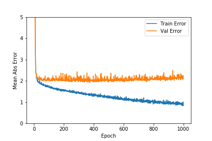
Plotting the Metrics

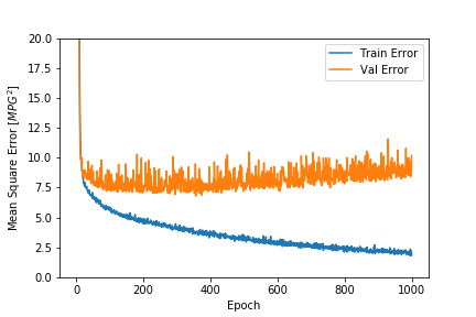
Let us plot the mean_squared_error, and mean_absolute_error to have better clarity of how our model performed.

hist = history.history

hist['epoch'] = history.epoch
plt.figure()
plt.xlabel('Epoch')
plt.ylabel('Mean Abs Error [MPG]')
plt.plot(hist['epoch'], hist['mean_absolute_error'],
         label='Train Error')
plt.plot(hist['epoch'], hist['val_mean_absolute_error'],
         label = 'Val Error')
plt.ylim([0,5])
plt.legend()
plt.savefig('Mean Abs Error.png')

plt.figure()
plt.xlabel('Epoch')
plt.ylabel('Mean Square Error [$MPG^2$]')
plt.plot(hist['epoch'], hist['mean_squared_error'],
         label='Train Error')
plt.plot(hist['epoch'], hist['val_mean_squared_error'],
         label = 'Val Error')
plt.ylim([0,20])
plt.legend()

plt.show()    

Evaluate the Model

Let’s see how our model performs on the unseen test data. This will give us a good idea of how our model will generalize when given real-world data.

loss, mae, mse = model.evaluate(norm_x_test, y_test, verbose=1)

print("Mean Abs Error: %.3f MPG" % (mae))

79/79 [==============================] - 0s 38us/step 
Mean Abs Error: 11.109 MPG

Predictions

We can now predict using the normalized test data that we have available with us.

preds = model.predict(norm_x_test).flatten()

To know better, we should plot the actual values and scatter plot of the predicted values.

plt.scatter(y_test, preds)
plt.xlabel('True Values')
plt.ylabel('Predictions')
plt.axis('equal')
plt.axis('square')
plt.xlim([0,plt.xlim()[1]])
plt.ylim([0,plt.ylim()[1]])
plt.plot([-100, 100], [-100, 100])
plt.savefig('predictions.png')

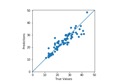
The predictions seem okay. Still, we can see a few outliers. Improvement can be done to the model by reducing the dimensionality of the second hidden layer and then analyzing the model performance. You should surely try that out on your own.

Summary and Conclusion

In this article, you learned how to perform regression using neural networks. You can try the above procedures on a new dataset of your choice as well.

If you liked this article, then please share and subscribe to the website. Leave your thoughts in the comment section. You can follow me on LinkedIn and Twitter as well.