
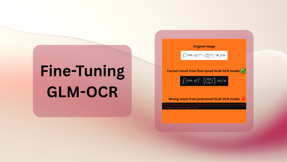
In the last article, we covered an introduction to GLM-OCR. The discussion revolved around the architecture and inference for various tasks. With specific prompts, along with text recognition, GLM-OCR can also carry out formula recognition. However, it falters in complex mathematical formulas. In this article, we will be fine-tuning GLM-OCR and observe to what extent we can improve the performance of the model on a task-specific dataset.
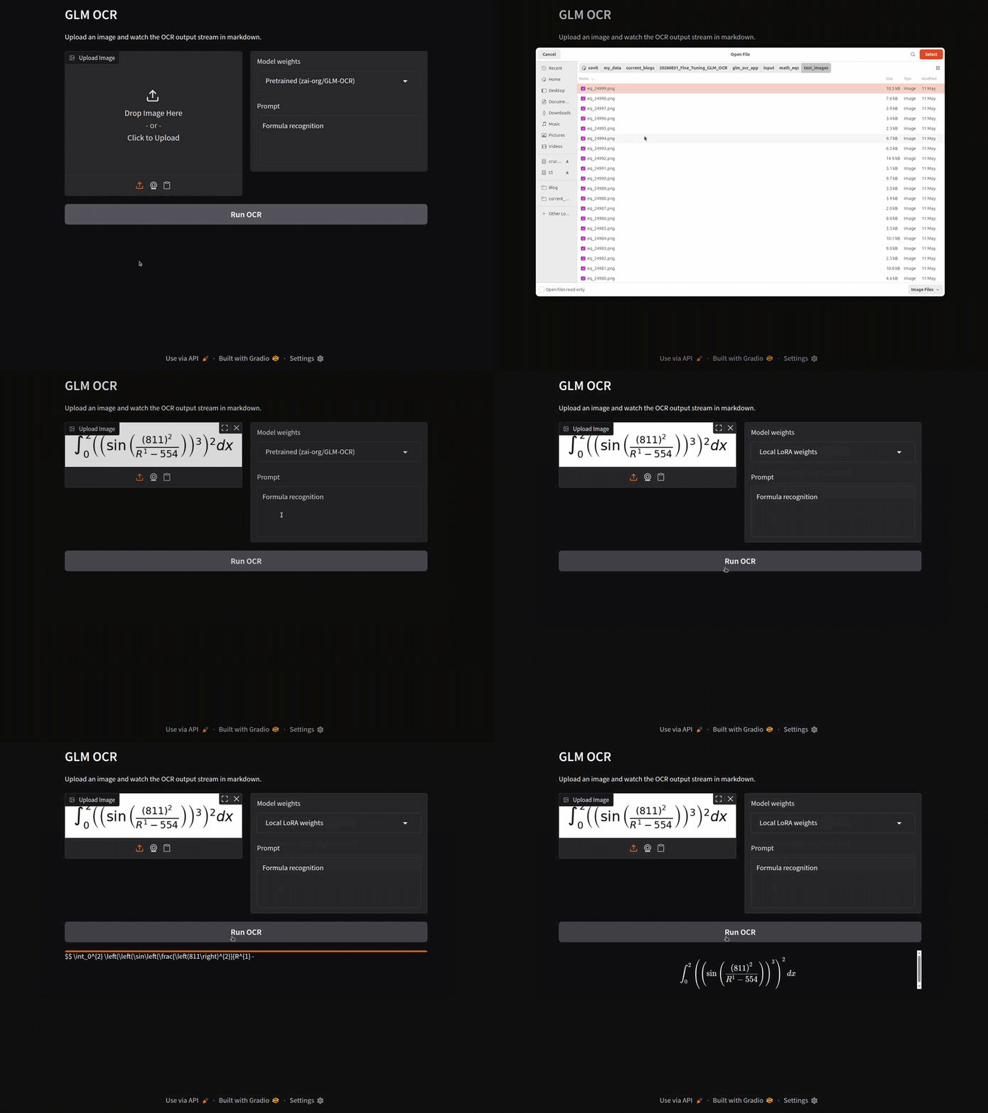
We will use a mathematical formula dataset for fine-tuning GLM-OCR here. It performs well on such samples out of the box. However, there are instances where the final OCR result is wrong, either because the formula is too complex or there are too many notations cluttered together. Our aim is to check whether fine-tuning on the entire dataset improves the results on such samples or not.
We will cover the following while training GLM-OCR:
- Understanding the mathematical formula dataset
- Setting up LLama-Factory for the training process
- Creating the dataset in the desired structure
- Fine-tuning the GLM-OCR model
- Creating a simple Gradio application for running inference
The Maths Equation Dataset
We will fine-tune the GLM-OCR model on the 25k_math_equation dataset from Kaggle.
The dataset contains images of 25000 mathematical equations along with their LaTeX equations in a text file.
We get the following directory structure after downloading and extracting the dataset.
├── images  [25000 entries exceeds filelimit, not opening dir]
└── labels.txt
The images directory contains the 25000 equation images and labels.txt file contains the LaTeX equations.
To understand the dataset better, let’s take a look at a few lines from the labels.txt file.
eq_00000.png	\int_0^{4} \left(y_{40}\right)^{1} dx
eq_00001.png	\sin\left(\frac{\ln\left(\frac{852}{479} \cdot P_{27}\right)}{\frac{\frac{\cos\left(M_{40}\right)}{\phi_{36}^{1} \cdot 459}}{\frac{\frac{u_{35}}{j^{7}}}{36}}}\right)
eq_00002.png	\cos\left(\frac{\frac{\left(Q^{1}\right)^{3}}{725 \cdot 12}}{\omega \cdot X - i^{10}} - \left(s_{14}\right) + \ln\left(z_{36}\right) - \left(l_{18} \cdot 695\right)^{5}\right)
Each new line contains two elements separated by a tab space. The first element is the image file name, and the second one is the LaTeX equation.
The following are a few image samples and their raw equations.
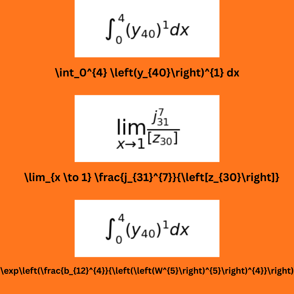
We can see that the dataset contains equations of varying complexity.
The Project Directory Structure
Let’s take a look at the project directory structure before moving into the codebase.
├── glm_ocr_app
│   ├── glm_ocr_lora_sft_math_eqs_data
│   │   ├── checkpoint-1000
│   │   │   ├── adapter_config.json
│   │   │   ├── adapter_model.safetensors
│   │   │   ├── chat_template.jinja
│   │   │   ├── optimizer.pt
│   │   │   ├── processor_config.json
│   │   │   ├── README.md
│   │   │   ├── rng_state.pth
│   │   │   ├── scheduler.pt
│   │   │   ├── tokenizer_config.json
│   │   │   ├── tokenizer.json
│   │   │   ├── trainer_state.json
│   │   │   └── training_args.bin
.
.
.
│   │   ├── adapter_config.json
│   │   ├── adapter_model.safetensors
│   │   ├── all_results.json
│   │   ├── chat_template.jinja
│   │   ├── processor_config.json
│   │   ├── README.md
│   │   ├── tokenizer_config.json
│   │   ├── tokenizer.json
│   │   ├── trainer_log.jsonl
│   │   ├── trainer_state.json
│   │   ├── training_args.bin
│   │   ├── training_loss.png
│   │   └── train_results.json
│   ├── input
│   │   └── math_eqs
│   │       ├── images  [24900 entries exceeds filelimit, not opening dir]
│   │       ├── test_images  [100 entries exceeds filelimit, not opening dir]
│   │       └── labels.txt
│   ├── gradio_app.py
│   ├── README.md
│   └── requirements.txt
├── LLaMA-Factory
│   ├── assets
│   │   ├── sponsors
│   │   │   ├── serpapi.svg
│   │   │   └── warp.jpg
│   │   ├── thirdparty
│   │   │   ├── colab.svg
│   │   │   ├── discord.svg
│   │   │   ├── dsw.svg
│   │   │   ├── lab4ai.svg
│   │   │   └── online.svg
│   │   └── logo.png
│   ├── data  [26 entries exceeds filelimit, not opening dir]
│   ├── docker
│   │   ├── docker-cuda
│   │   │   ├── docker-compose.yml
│   │   │   ├── Dockerfile
│   │   │   ├── Dockerfile.base
│   │   │   ├── Dockerfile.megatron
│   │   │   └── README.md
│   │   ├── docker-npu
│   │   │   ├── docker-compose.yml
│   │   │   └── Dockerfile
│   │   └── docker-rocm
│   │       ├── docker-compose.yml
│   │       └── Dockerfile
│   ├── docs
│   │   ├── en
.
.
.
│   │   │   ├── hyperparameters
│   │   │   │   ├── data-argument.md
│   │   │   │   ├── model-argument.md
│   │   │   │   ├── sample-argument.md
│   │   │   │   └── training-argument.md
│   │   │   ├── inference
│   │   │   │   └── deploy.md
.
.
.
└── README.md
- We have two main directories. One is the
glm_ocr_appthat contains the Gradio application script for testing the fine-tuned model. Along with that, it also contains theglm_ocr_lora_sft_math_eqs_datathat contains the fine-tuned LoRA so that we can load it easily when running the test experiments. - Then we have the
LLaMA-Factorydirectory which will be our primary working ground for preparing the dataset and fine-tuning. We are using the LlamaFactory repository here to handle the training process.
We will get into the setup steps in the next section.
The article comes with a zip file containing the dataset preprocessing script, the Gradio inference script, and the fine-tuned LoRA. The following sections explain how to handle the directory structure and where to copy the necessary files to carry on with the article.
Download Code
Exploring the Codebase for Fine-Tuning GLM-OCR
Let’s jump into the coding section for this article. We will cover the following here:
- Dataset preparation for training the GLM-OCR model
- Training the model
- Inference using the trained LoRA model
Before moving further, please download the zip file that comes with this article, as we will need the dataset preparation script from there.
Setting Up Llama-Factory
Let’s set up LLaMA-Factory first. These steps are almost identical to the ones provided in the official GLM-OCR repository. The only changes are going to be our dataset preparation steps. Clone the repository and install the requirements.
git clone --depth 1 https://github.com/hiyouga/LLaMA-Factory.git
cd LLaMA-Factory
pip install -e .
pip install -r requirements/metrics.txt
pip install peft==0.19.1
Next, install the latest version of Transformers.
pip install --upgrade transformers
In case you face issues, install the pinned version that was used for the codebase of this article.
pip install transformers==5.6.0
Dataset Preparation
Next comes the crucial part, preparing the training dataset.
First, copy the mathematical equation dataset that we previously downloaded into the data directory inside the LLaMA-Factory repository. The full path will be LLaMA-Factory/data.
We have renamed the mathematical equation directory to math_eqs for easier access, and it contains the images subdirectory and the labels.txt file.
Second, the zip file that comes with the article contains a dataset preparation script, prepare_math_eqs_data.py. Copy the same to the LLaMA-Factory/data directory. Finally, the directory should look similar to the following.

Let’s take a look at prepare_math_eqs_data.py script.
import os
import json

from tqdm import tqdm

DATA_ROOT_DIR = 'math_eqs'
IMAGE_PATH = os.path.join(DATA_ROOT_DIR, 'images')
LABEL_PATH = os.path.join(DATA_ROOT_DIR, 'labels.txt')

def prepare_math_eqs_data(image_dir_path, label_path):
    """
    The text file contains the separate lines in this format.

    eq_00000.png	\int_0^{4} \left(y_{40}\right)^{1} dx

    The image file name and the equation is separated by tab-space.
    """

    data = []
    with open(label_path, 'r', encoding='utf-8') as f:
        labels_data = f.read().strip().splitlines()

    for i, line in enumerate(tqdm(labels_data, desc="Processing labels")):
        image_name, formula_text = line.split('\t')
        image_path = os.path.join(image_dir_path, image_name)

        if os.path.exists(image_path):
            data.append({
                    "messages": [
                        {
                            "role": "user",
                            "content": "Formula recognition:"
                        },
                        {
                            "role": "assistant",
                            "content": f"\$$ {formula_text} \$$"
                        }
                    ],
                    "images": [image_path]
                })
        else:
            print(f"Warning: Image file {image_path} does not exist.")

    return data

if __name__ == '__main__':

    data = prepare_math_eqs_data(IMAGE_PATH, LABEL_PATH)
    output_file = 'math_eqs_data.json'
    with open(output_file, 'w', encoding='utf-8') as f:
        json.dump(data, f, ensure_ascii=False, indent=4)

    print(f"Data preparation complete. JSON file saved as {output_file}.")
This creates a math_eqs_data.json in the LLaMA-Factory/data directory in the ShareGPT format. We extract the image names and the raw LaTeX equations from the math_eqs/labels.txt file by splitting the data into separate lines. Then we get the relative image path from math_eqs/images directory and create the JSON file in the following structure.
[
  {
    "messages": [
      {
        "role": "user",
        "content": "Formula recognition:"
      },
      {
        "role": "assistant",
        "content": "\$\$\$\$"
      }
    ],
    "images": [
      "math_eqs/images/eq_00000.png"
    ]
  },
  {
    "messages": [
      {
        "role": "user",
        "content": "Formula recognition:"
      },
      {
        "role": "assistant",
        "content": "\$\$\$\$"
      }
    ],
    "images": [
      "math_eqs/images/eq_00000.png"
    ]
  }
  ...
]
We enclose the equations within the $$ signs so that the model learns to generate the equations in one shot.
We can execute the script within the LLaMA-Factory/data directory to generate the math_eqs_data.json file.
python prepare_math_eqs_data.py
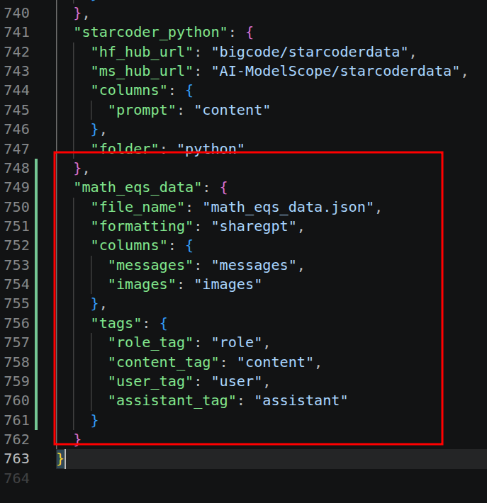
Next, we need to register the dataset JSON file in the LLaMA-Factory/data/dataset_info.json file. It already contains a number of pre-registered datasets. We can register our own dataset at the end of the JSON structure.
"math_eqs_data": {
    "file_name": "math_eqs_data.json",
    "formatting": "sharegpt",
    "columns": {
      "messages": "messages",
      "images": "images"
    },
    "tags": {
      "role_tag": "role",
      "content_tag": "content",
      "user_tag": "user",
      "assistant_tag": "assistant"
    }
  }
It should look like the following.
Training the GLM-OCR Model
We will carry out LoRA fine-tuning of the GLM-OCR model here. The zip file that comes with this article also contains a glm_ocr_lora_sft.yaml. This is a modified training configuration file from the GLM-OCR repository. Copy and paste this into the parent LLaMA-Factory directory.
The following is the content of the file.
### model
model_name_or_path: zai-org/GLM-OCR    # or local path: /path/to/GLM-OCR
trust_remote_code: true

### method
stage: sft
do_train: true
finetuning_type: lora
lora_rank: 16
lora_target: all

### dataset
dataset: math_eqs_data
template: glm_ocr
cutoff_len: 2048
max_samples: 25000
preprocessing_num_workers: 8
dataloader_num_workers: 4

### output
output_dir: ./glm_ocr_lora_sft_math_eqs_data
logging_steps: 10
save_steps: 1000
plot_loss: true
overwrite_output_dir: true
save_only_model: false
report_to: none  # choices: [none, wandb, tensorboard, swanlab, mlflow]

### train
per_device_train_batch_size: 8
gradient_accumulation_steps: 4
learning_rate: 1.0e-4
num_train_epochs: 5
lr_scheduler_type: cosine
warmup_ratio: 0.1
bf16: true
ddp_timeout: 180000000
resume_from_checkpoint: null

### eval
# val_size: 0.1
# per_device_eval_batch_size: 1
# eval_strategy: steps
# eval_steps: 500
Although there are several parameters in the above YAML file, a few are quite important:
finetuning_type: lora: This tells the training script that we want to carry out a LoRA fine-tuning.lora_rank: 16andlora_target: all: We are using a LoRA rank of 16, and we are training all the linear weights in the adapter.max_samples: 25000: We will be training the model on all 25000 samples.preprocessing_num_workers: 8anddataloader_num_workers: 4: 8 CPU workers will be used for tokenizing the dataset, and 4 will be used for the dataloader.- Finally, we are using a batch size of 8, with 4 gradient accumulation steps, and training for 5 epochs.
The above training setting uses 6 GB-7 GB of VRAM.
All the training and inference experiments shown here were carried out on a 10GB RTX 3080 GPU.
Let’s start the training process now. We will execute the following command within the Llama-Factory directory to start the training.
DISABLE_VERSION_CHECK=1 CUDA_VISIBLE_DEVICES=0 llamafactory-cli train glm_ocr_lora_sft.yaml
The adapter checkpoints will be saved in the glm_ocr_lora_sft_math_eqs_data directory.
The following are the training logs and the training loss graph.
{
    "epoch": 5.0,
    "total_flos": 1.4272293267033293e+17,
    "train_loss": 0.05630928651641702,
    "train_runtime": 4554.0756,
    "train_samples_per_second": 27.448,
    "train_steps_per_second": 0.859
}
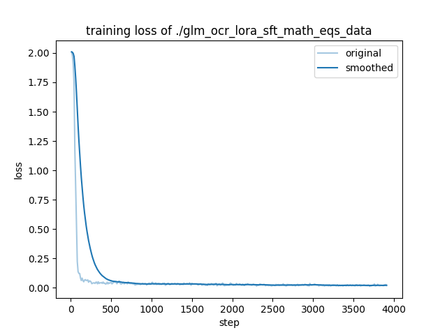
Although the loss is low, we will get more insights once we run inference using the trained adapter.
Running Inference Using the Trained GLM-OCR Adapter
We have the gradio_app.py script in the glm_ocr_app directory. The file launches a Gradio application where we can either load the pretrained GLM-OCR model or our trained adapter model for running inference.
Let’s start the application and check a few results.
python gradio_app.py
The following video shows a workflow where we load the LoRA weights and run inference.
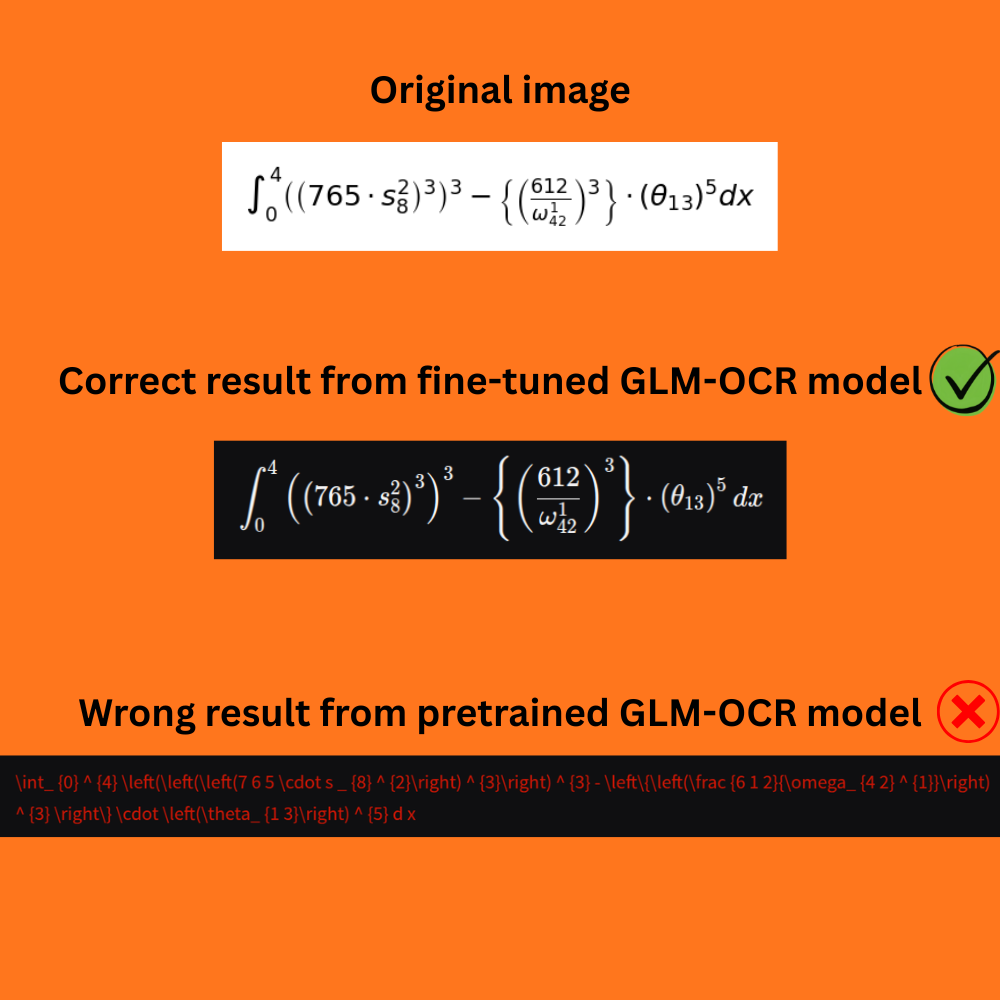
Now, the real question is whether our fine-tuning process made an impact or not. To some extent, it did. For example, the following figure shows an original image (eq_24981.png), where the pretrained model gave a malformed LaTeX formula, and the fine-tuned one generated the correct equation.
However, there are some extremely complex samples like eq_24990.png and eq_24984.png where, even after fine-tuning, although some of the notations were generated correctly, the final formula was not entirely correct.
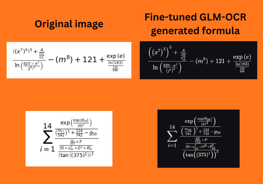
There could be several reasons for this. Maybe we need even more training data. Or perhaps the notations are so small and unclear that the model is unable to learn the features. However, training on even more high-quality and high-resolution data will surely solve this.
Summary and Conclusion
In this article, we focused on fine-tuning the GLM-OCR model on a mathematical equation dataset. We started with the dataset exploration, moved to preparing the dataset in ShareGPT format, and carried out training & inference. We also discussed where the trained adapter needs improvement. I hope this article was worth your time.
If you have any questions, thoughts, or suggestions, please leave them in the comment section. I will surely address them.
You can contact me using the Contact section. You can also find me on LinkedIn, and X.