Multi-Label Fashion Item Classification using Deep Learning and PyTorch

In this tutorial, you will get to learn how to carry out multi-label fashion item classification using deep learning and PyTorch. We will use a pre-trained ResNet50 deep learning model to apply multi-label classification to the fashion items.

For the training and validation, we will use the Fashion Product Images (Small) dataset from Kaggle. We will come back to the dataset a bit later.

Before moving forward, I highly recommend that you go through a few previous articles. These will help you if you are new to multi-label classification and multi-head neural networks in deep learning.

• Multi-Label Image Classification with PyTorch and Deep Learning.
• Multi-Head Deep Learning Models for Multi-Label Classification.
• Deep Learning Architectures for Multi-Label Classification using PyTorch.

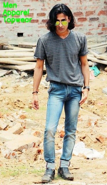
Figure 1 shows how our multi-label fashion item classification is going to look like. We will classify each fashion item image into three classes, just like the above image.

So, what are we going to do specifically in this article?

• Downloading the Fashion Product Images (Small) dataset and exploring it to know about the images and labels.
• Getting into the code part, fine-tuning a pre-trained ResNet50 neural network model. We will load the pre-trained weights and add multiple heads for multi-label classification. Then we will re-train it on our own dataset to carry out multi-label fashion item classification using deep learning and PyTorch.
• We will train and validate the model for 20 epochs.
• Finally, we will run inference to test the trained model on totally new images.

I hope that you are excited to follow along this article.

About the Fashion Images Dataset that We Will Use

We will use the Fashion Product Images (Small) from Kaggle for this tutorial. This dataset contains more than 44000 images and the dataset size is somewhere around 545 MB. So, it is reasonable enough for a blog post. This dataset is actually a mini version of the original Fashion Product Images on Kaggle which contains much higher resolution images. That dataset is really huge, that is, 23 GB. Obviously, the small version that we will be using is a much better use-case for this tutorial.

Images and Labels in the Dataset

Now, we know that we will be carrying out multi-label classification using deep learning in this tutorial. But what do the labels for a single image look like in this dataset? Let’s explore that a bit.

The following image shows a few rows from the CSV of the dataset.

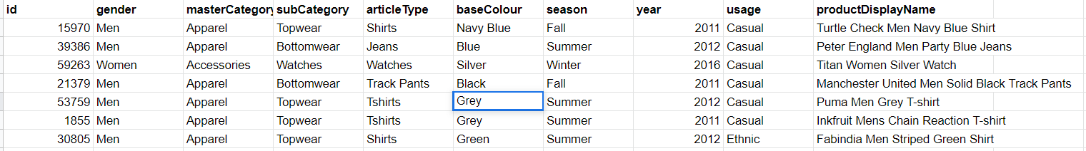
In figure 2, we have 10 columns in total. The first one, that is id corresponds to the image id that our dataset contains. All the other columns after that are the labels for that image. But we can see that there many columns (9 in total). And we have even a year column which we obviously don’t need for classification.

So, how are we going to approach out multi-label fashion item classification using deep learning?

To make matters a bit simpler and yet keep the learning curve to a certain standard, we will consider the first three label columns. They are gender, masterCategory, and subCategory. This is going to be plenty for learning about a real-world dataset multi-label classification using deep learning.

Also, we can see that the labels are not binary. Each label contains different categories in themselves. So, what are all the unique categories in each of the three labels that we will be using? The following snippet should give you a good idea.

Gender values: ['Men' 'Women' 'Boys' 'Girls' 'Unisex'], Total 5
Master category values: ['Apparel' 'Accessories' 'Footwear' 'Personal Care' 'Free Items'
 'Sporting Goods' 'Home'], Total 7
Sub category values: ['Topwear' 'Bottomwear' 'Watches' 'Socks' 'Shoes' 'Belts' 'Flip Flops'
 'Bags' 'Innerwear' 'Sandal' 'Shoe Accessories' 'Fragrance' 'Jewellery'
 'Lips' 'Saree' 'Eyewear' 'Nails' 'Scarves' 'Dress'
 'Loungewear and Nightwear' 'Wallets' 'Apparel Set' 'Headwear' 'Mufflers'
 'Skin Care' 'Makeup' 'Free Gifts' 'Ties' 'Accessories' 'Skin'
 'Beauty Accessories' 'Water Bottle' 'Eyes' 'Bath and Body' 'Gloves'
 'Sports Accessories' 'Cufflinks' 'Sports Equipment' 'Stoles' 'Hair'
 'Perfumes' 'Home Furnishing' 'Umbrellas' 'Wristbands' 'Vouchers'], Total 45

The gender label contains 5 categories in total. The masterCategory label contains 7 categories in total. And the subCategory contains 45 categories in total. Looks like this is going to be a good challenge for us and also for the ResNet50 deep learning network to tackle this one.

Now, coming to the images. All of them are pretty small with a resolution of 60×80 (mostly). This is the reason the dataset is around 545 MB even with 44000 images.

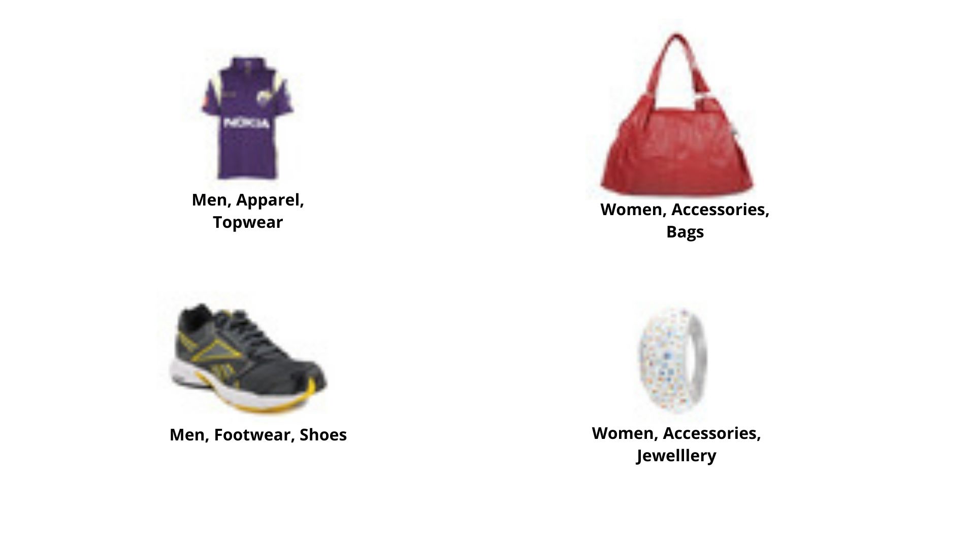
Figure 3 shows a few of the fashion items with the categories corresponding to the three labels that we will be using.

We will try our best to train a neural network model well to do the multi-label classification for us.

The Directory Structure

In this section, we will set up our directory structure that we will use for this project. Take a look at the following snippet.

├───input
│   ├───fashion-product-images-small
│   │   │   styles.csv
│   │   │
│   │   ├───images
│   │   │       10000.jpg
│   │   │       10001.jpg
│   │   │       10002.jpg
|   |   |       ...
│   └───test_data
├───outputs
└───src
    │   dataset.py
    │   label_dicts.py
    │   loss_functions.py
    │   models.py
    │   test.py
    │   train.py
    │   utils.py

First, we need to download the Fashion Product Images (Small) dataset and extract it inside the input folder.

• The input folder has the fashion-product-images-small subfolder which contains the styles.csv file. It also contains the images folder which holds all the fashion item images. Note: You may find another myntradataset folder which you can safely ignore. This is just the repeatition of the entire dataset again. The input folder also contains the test_data folder which has all the images that we will use for testing our trained model in the end.
• Then we have the outputs folder that will contain all the outputs that will be generated during training and testing. This includes the trained model weights, the loss plots, and the final output images after testing.
• Finally, we have the src folder which contains 7 Python code files. We will get into the details of these while writing the code.

Now, coming to the test data. You can choose any image from the internet or you can use the same images that I will be using. If you want to use the same test images as this tutorial, then you can download them from below.

After downloading the file, just extract it inside the input folder. All these images are take from Pixabay and free to use.

Important Libraries and Frameworks

First of all, we will be using the PyTorch deep learning framework for all the neural network and deep learning stuff in this tutorial. All the code is written with PyTorch 1.6. Older or newer versions might work as well, but they are not tested as of now.

Secondly, you will need the Joblib to some extent as well. Please install it before moving forward if you do not have it already.

We will use the ResNet50 neural network for training on this dataset. I am using the Pretrained models for Pytorch library to load and finetune the model. This is a great open-source project which contains a lot of pre-trained vision models for PyTorch. We can load any of these and fine-tune them according to our dataset. You need to install this if you do not have it already. You can easily install using the pip command.

pip install pretrainedmodels

If you want, you can also start contributing to the project and show your support by starring it as well.

All the other libraries, mostly you will have them if you are into machine learning and deep learning. Along the way, if you notice you are missing anything, feel free to install them.

Multi-Label Fashion Item Classification using Deep Learning and PyTorch

Before moving further: The images in the dataset might be small, but it is a big dataset. It contains more than 44000 images. For this reason, the training can take a lot of time to complete if you run this on a CPU or a mid-range GPU. Therefore, I have curated a Kaggle kernel containing the whole training code. You are free to fork this kernel and run it on your own as well if you have any hardware resource constraint. If you have adequate compute power, you are free to code along on your local machine.

From here onward, we will start with the coding part of this tutorial. We will tackle each Python file in its respective section.

Writing the Utility Functions

We will start with writing some utility and helper functions. These are mainly for cleaning the data, saving the trained model, and saving the loss plots.

We will write all these utility functions inside the utils.py Python file.

Let’s start with the imports that we will need along the way for the utility functions.

import os
import torch
import matplotlib.pyplot as plt
import matplotlib

from tqdm import tqdm

matplotlib.style.use('ggplot')

We will need torch for writing the function to save our trained model weights. And matplotlib is for the function that we will use to save the loss plot with.

Function to Clean the Data

In our dataset, we have the images folder which contains the fashion item images. The styles.csv contains the image ids along with the labels that image belongs to. But some images corresponding to the image ids from the CSV file are missing in the images folder. This will surely cause issues while trying to read that particular image while training.

So, if an image is not present, then we will remove that image id from the CSV file as well. That’s what clean_data() function will do. The following code block contains the function definition.

def clean_data(df):
    """
    this functions removes those rows from the DataFrame for which there are
    no images in the dataset
    """
    drop_indices = []
    print('[INFO]: Checking if all images are present')
    for index, image_id in tqdm(df.iterrows()):
        if not os.path.exists(f"../input/fashion-product-images-small/images/{image_id.id}.jpg"):
            drop_indices.append(index)

    print(f"[INFO]: Dropping indices: {drop_indices}")
    df.drop(df.index[drop_indices], inplace=True)
    return df

• First of all, this function accepts the CSV file as a DataFrame.
• From line 16, we have a for loop going over all the rows in the CSV file. If we do not find an image corresponding to the image id in the images folder, then we add that index to the drop_indices list.
• At line 21, we drop those indices from the DataFrame and then we return the new DataFrame.

After doing this, we should not be facing any error while reading the images from the folder.

Function to Save the Model

We will write a simple function to save the trained model weights to the disk. The following code block contains the function.

# save the trained model to disk
def save_model(epochs, model, optimizer, criterion):
    torch.save({
                'epoch': epochs,
                'model_state_dict': model.state_dict(),
                'optimizer_state_dict': optimizer.state_dict(),
                'loss': criterion,
                }, '../outputs/model.pth')

• The save_model() accepts the number of epochs, the model, the optimizer, and the criterion (loss function) as parameters.
• We use the torch.save() function to save each detail along with the trained weights as a dictionary. We save this in the outputs folder.

Function to Save the Loss Plots

Finally, we will write another function to save the loss plots for training and validation.

# save the train and validation loss plots to disk
def save_loss_plot(train_loss, val_loss):
    plt.figure(figsize=(10, 7))
    plt.plot(train_loss, color='orange', label='train loss')
    plt.plot(val_loss, color='red', label='validataion loss')
    plt.xlabel('Epochs')
    plt.ylabel('Loss')
    plt.legend()
    plt.savefig('../outputs/loss.jpg')
    plt.show()

We use the train_loss and val_loss lists to save the loss line graphs to disk. We will get these two lists while training and validating our deep learning model on the dataset.

Preparing the Label Dictionaries

In one of the previous sections, we have seen the labels for the gender, masterCategory, and subCategory. Each of the labels have 5, 7, and 45 categories respectively. But all of them are in the text format which we cannot feed into our deep neural network.

To be able to feed all of those category labels into our neural network while training we need them as numbers (0, 1, 2, …). That’s what we are going to do in this section. We will create three dictionaries that will map the text categories to numbers. Then we will save those to disk as .pkl files as well, so that we can load them whenever we want.

All the code in this section will go into label_dicts.py file.

The following are the imports that we will need for the code.

import pandas as pd
import joblib

from utils import clean_data

• We are importing joblib here which will help us to save the dictionaries as .pkl files.
• Also, we are importing the clean_data function from utils that we have written in the previous section.

Function to Map the Categories to Numbers and Save Them

We will write a save_label_dicts() function which will accept the DataFrame containing all the image ids and labels as parameters. Let’s get into the code first, then we will move on to the explanation part.

def save_label_dicts(df):
    # remove rows from the DataFrame which do not have corresponding images
    df = clean_data(df)

    # we will use the `gender`, `masterCategory`. and `subCategory` labels
    # mapping `gender` to numerical values
    cat_list_gender = df['gender'].unique()
    # 5 unique categories for gender
    num_list_gender = {cat:i for i, cat in enumerate(cat_list_gender)}
    # mapping `masterCategory` to numerical values
    cat_list_master = df['masterCategory'].unique()
    # 7 unique categories for `masterCategory`
    num_list_master = {cat:i for i, cat in enumerate(cat_list_master)}
    # mapping `subCategory` to numerical values
    cat_list_sub = df['subCategory'].unique()
    # 45 unique categories for `subCategory`
    num_list_sub = {cat:i for i, cat in enumerate(cat_list_sub)}

    joblib.dump(num_list_gender, '../input/num_list_gender.pkl')
    joblib.dump(num_list_master, '../input/num_list_master.pkl')
    joblib.dump(num_list_sub, '../input/num_list_sub.pkl')

df = pd.read_csv('../input/fashion-product-images-small/styles.csv', usecols=[0, 1, 2, 3, 4, 4, 5, 6, 9])
save_label_dicts(df)

• First, the most important step is cleaning the DataFrame. We are doing that at line 7. This removes all the rows from the DataFrame which do no have the corresponding images in the dataset.
• Then we move on to create three dictionary mapping from categories to numbers. We start with the gender label at line 11. Here, cat_list_gender stores all the unique categories that we have for the label (men, women, and so on). Then at line 13, we create a dictionary that maps all the text categories to numerical values.
• We take similar steps for the masterCategory and subCategory labels from lines 15 to 21.
• Coming to lines 23 to 25, we are saving all the three dictionary mappings as serialized pickle files to disk.
• At line 27, we read the styles.csv from disk. We also use the usecols argument to specify that we only need the first 10 columns. I have done this as sometimes the texts in the last column in the CSV file were overflowing to the next column which does not have any header. This results in an error which we can prevent by using usecols.
• Finally, we are calling the save_label_dicts() function.

Now, we also need to execute the label_dicts.py python script to save the pickle files to disk. Open up your command prompt/terminal, cd into the src folder, and type the following command.

python label_dicts.py

You should see the following output.

[INFO]: Checking if all images are present
44446it [00:29, 1501.41it/s]
[INFO]: Dropping indices: [6697, 16207, 32324, 36399, 40022]

You may also print the text to number dictionary mappings. That should give you the following result.

{'Men': 0, 'Women': 1, 'Boys': 2, 'Girls': 3, 'Unisex': 4}

{'Apparel': 0, 'Accessories': 1, 'Footwear': 2, 'Personal Care': 3, 'Free Items': 4, 'Sporting Goods': 5, 'Home': 6}

{'Topwear': 0, 'Bottomwear': 1, 'Watches': 2, 'Socks': 3, 'Shoes': 4, 'Belts': 5, 'Flip Flops': 6, 'Bags': 7, 'Innerwear': 8, 'Sandal': 9, 'Shoe Accessories': 10, 'Fragrance': 11, 'Jewellery': 12, 'Lips': 13, 'Saree': 14, 'Eyewear': 15, 'Nails': 16, 'Scarves': 17, 'Dress': 18, 'Loungewear and Nightwear': 19, 'Wallets': 20, 'Apparel Set': 21, 'Headwear': 22, 'Mufflers': 23, 'Skin Care': 24, 'Makeup': 25, 'Free Gifts': 26, 'Ties': 27, 'Accessories': 28, 'Skin': 29, 'Beauty Accessories': 30, 'Water Bottle': 31, 'Eyes': 32, 'Bath and Body': 33, 'Gloves': 34, 'Sports Accessories': 35, 'Cufflinks': 36, 'Sports Equipment': 37, 'Stoles': 38, 'Hair': 39, 'Perfumes': 40, 'Home Furnishing': 41, 'Umbrellas': 42, 'Wristbands': 43, 'Vouchers': 44}

This gives us a clear picture of what is happening.

Preparing the Dataset

One of the most important steps in deep learning, preparing the dataset.

We need to create our image dataset class which will provide us with the training and validation dataset. In turn, we will use those to get the training and validation data loaders for PyTorch training.

We will create our dataset class in this section. We will write this code inside the dataset.py Python file.

Let’s check all the Python imports that we will need for dataset code.

from torch.utils.data import Dataset
from utils import clean_data

import torch
import joblib
import math
import cv2
import torchvision.transforms as transforms

Some of the important import statements:

• We are importing the clean_data function from utils that we will use to clean the DataFrame.
• joblib will help us load the serialized dictionaries that we have saved to disk.
• We will need cv2 for reading images.
• Also, we will need to transforms from torchvision to apply image transforms and augmentations as well.

Split the DataFrame into Training and Validation Set

We need a training dataset and a validation dataset for training and validation respectively.

To do that split, we will write a simple function, train_val_split() that accepts the original DataFrame. Following is the code for that.

def train_val_split(df):
    # remove rows from the DataFrame which do not have corresponding images
    df = clean_data(df)

    # shuffle the dataframe
    df = df.sample(frac=1).reset_index(drop=True)

    # 90% for training and 10% for validation
    num_train_samples = math.floor(len(df) * 0.90)
    num_val_samples = math.floor(len(df) * 0.10)

    train_df = df[:num_train_samples].reset_index(drop=True)
    val_df = df[-num_val_samples:].reset_index(drop=True)

    return train_df, val_df

• The first step is to clean the DataFrame of image ids for which there are no images. We are doing that at line 11.
• After that, we are shuffling the DataFrame and splitting it into a 90% training set and 10% validation set (lines 14 to 21).
• Lines 20 and 21 also reset the index values of train_df and val_df so that both of them have index positions starting from one.
• Finally, we return the training and validaiton DataFrames.

The Fashion Dataset Class

Now, we will move on to write the dataset class that we need.

I am including the whole dataset class in the following code block, then we will get into the explanation part.

class FashionDataset(Dataset):
    def __init__(self, df, is_train=True):
        self.df = df
        self.num_list_gender = joblib.load('../input/num_list_gender.pkl')
        self.num_list_master = joblib.load('../input/num_list_master.pkl')
        self.num_list_sub = joblib.load('../input/num_list_sub.pkl')
        self.is_train = is_train

        # the training transforms and augmentations
        if self.is_train:
            self.transform = transforms.Compose([
                transforms.ToPILImage(),
                transforms.Resize((224, 224)),
                transforms.RandomHorizontalFlip(p=0.5),
                transforms.RandomVerticalFlip(p=0.5),
                transforms.ToTensor(), 
                transforms.Normalize(mean=[0.485, 0.456, 0.406],
                                     std=[0.229, 0.224, 0.225])
            ])

        # the validation transforms
        if not self.is_train:
            self.transform = transforms.Compose([
                transforms.ToPILImage(),
                transforms.Resize((224, 224)),
                transforms.ToTensor(),
                transforms.Normalize(mean=[0.485, 0.456, 0.406],
                                     std=[0.229, 0.224, 0.225])
            ])

    def __len__(self):
        return len(self.df)

    def __getitem__(self, index):
        image = cv2.imread(f"../input/fashion-product-images-small/images/{self.df['id'][index]}.jpg")
        image = cv2.cvtColor(image, cv2.COLOR_BGR2RGB)
        image = self.transform(image)

        cat_gender = self.df['gender'][index]
        label_gender = self.num_list_gender[cat_gender]

        cat_master = self.df['masterCategory'][index]
        label_master = self.num_list_master[cat_master]

        cat_sub = self.df['subCategory'][index]
        label_sub = self.num_list_sub[cat_sub]

        # image to float32 tensor
        image = torch.tensor(image, dtype=torch.float32)
        # labels to long tensors
        label_gender = torch.tensor(label_gender, dtype=torch.long)
        label_master = torch.tensor(label_master, dtype=torch.long)
        label_sub = torch.tensor(label_sub, dtype=torch.long)

        return {
            'image': image,
            'gender': label_gender,
            'master': label_master,
            'sub': label_sub
        }

Let’s start with the __init__() method.

• This accepts the DataFrame and one is_train variable as argument. We will use is_train to know whether to apply train augmentations or validation augmentations.
• We initialize the is_train and DataFrame.
• Along with that we also read and initialize the pickled and serialized category to number dictionaries from the disk at lines 27, 28, and 29.
• At line 33, we define the training augmentations and transforms if is_train is True. Along with resizing all the images to 224×224 dimension, we are also applying random horizontal and vertical flips to the images. We are also applying the ImageNet normalization values as we will be using a ResNet50 network that has been pre-trained on the ImageNet dataset.
• If is_train is False, then we apply the validation transforms. This does not include any image augmentation, just the general image transforms.

Now coming to the __getitem__() method.

• Lines 58, 59, and 60 read the image, convert the image to RGB color format, and apply the image transforms respectively.
• The next few lines are a bit important. At line 62, we get the category name (word) from the gender label column. It could be Men, Women, or any one of the 5 categories. Then at line 63, we map this category (acting as the key) to the numerical value that is stored in the num_list_gender dictionary. This gives us a numerical value that will act as the target label while training. We repeat this step for the masterCategory and subCategory labels as well (lines 65 to 69).
• Starting from line 72, we convert the image into float32 tensor and all the labels into long tensors.
• Finally, we return the image tensors and all the label tensors in the form of a dictionary.

This completes the dataset class that we need to prepare training and validation datasets.

The Loss Function

We have to write a custom function for the loss function. This is because we have three different labels for which we will have three different loss values in each iteration while training. Therefore, we will need to average over the three loss values.

We will write our custom loss function in the loss_functions.py Python file.

import torch.nn as nn

# custom loss function for multi-head multi-category classification
def loss_fn(outputs, targets):
    o1, o2, o3 = outputs
    t1, t2, t3 = targets
    l1 = nn.CrossEntropyLoss()(o1, t1)
    l2 = nn.CrossEntropyLoss()(o2, t2)
    l3 = nn.CrossEntropyLoss()(o3, t3)

    return (l1 + l2 + l3) / 3

The loss_fn() accepts the outputs and targets as tuples. We extract the values from those at lines 5 and 6. Then we calculate three loss values using the output labels, and the target labels. We use the Cross-Entropy loss function as we have more than 1 category for each of the labels. Finally, we average over the loss values and return the final value.

You can also learn more about such loss functions in this article.

The Deep Learning Model

As discussed earlier, we will use a ResNet50 deep learning model trained on the ImageNet dataset. We will change the network classification heads according to our use-case and dataset.

I hope that you have already installed the Pretrained models for Pytorch library before moving further.

This code will into the models.py Python file.

We need three imports preparing our deep learning model.

import torch.nn as nn
import torch.nn.functional as F
import pretrainedmodels

The following code block contains the whole model class code.

class MultiHeadResNet50(nn.Module):
    def __init__(self, pretrained, requires_grad):
        super(MultiHeadResNet50, self).__init__()
        if pretrained == True:
            self.model = pretrainedmodels.__dict__['resnet50'](pretrained='imagenet')
        else:
            self.model = pretrainedmodels.__dict__['resnet50'](pretrained=None)

        if requires_grad == True:
            for param in self.model.parameters():
                param.requires_grad = True
            print('Training intermediate layer parameters...')
        elif requires_grad == False:
            for param in self.model.parameters():
                param.requires_grad = False
            print('Freezing intermediate layer parameters...')

        # change the final layers according to the number of categories
        self.l0 = nn.Linear(2048, 5) # for gender
        self.l1 = nn.Linear(2048, 7) # for masterCategory
        self.l2 = nn.Linear(2048, 45) # for subCategory

    def forward(self, x):
        # get the batch size only, ignore (c, h, w)
        batch, _, _, _ = x.shape
        x = self.model.features(x)
        x = F.adaptive_avg_pool2d(x, 1).reshape(batch, -1)
        l0 = self.l0(x)
        l1 = self.l1(x)
        l2 = self.l2(x)
        return l0, l1, l2

• The __init__() method receives two parameters, pretrained and requires_grad. While training, we will provide pretrained=True and requires_grad=False. This will ensure that all the ImageNet weights are loaded and the intermediate layer parameters are frozen. We will only add our custom classification heads which will be learnable.
• Starting from line 22, we add three learnable classification heads. Each of the self.l0, self.l1, and self.l2 are for classifying the gender, masterCategory, and subCategory respectively. The output features correspond to the number of categories in each of those labels.
• In the forward() function, first, we get a hold of the pre-trained features at line 29. Then we flatten the features before feeding them to each of the linear classification heads in the subsequent lines.
• Finally, we return the outputs from the three linear classification heads.

This is all we need for preparing the deep learning model.

The Training Code

Here, we will start writing the training code for training our multi-head ResNet50 model on the Fashion Images dataset.

We will write the training code inside the train.py Python file.

First of all, the import that we need.

import pandas as pd
import torch
import torch.optim as optim

from dataset import train_val_split, FashionDataset
from torch.utils.data import DataLoader
from models import MultiHeadResNet50
from tqdm import tqdm
from loss_functions import loss_fn
from utils import save_model, save_loss_plot

Going over a few important imports here.

• We are importing the train_val_split function, and the FashionDataset class from dataset.
• From models we are importing our custom multi-head ResNet50 deep learning model.
• We are also importing our custom loss function and functions to save the trained model weights and the loss plot as well.

Define the Computation Device, Initialize the Model, and Set the Learning Parameters

For the computation device, here, we almost have no other choice other than using a GPU. I highly recommend that you should have a GPU for training on your own system.

The following code block defines the computation device, initializes the model, and sets the learning parameters as well.

# define the computation device
device = torch.device('cuda' if torch.cuda.is_available() else 'cpu')
# initialize the model
model = MultiHeadResNet50(pretrained=True, requires_grad=False).to(device)

# learning parameters
lr = 0.001
optimizer = optim.Adam(params=model.parameters(), lr=lr)
criterion = loss_fn
batch_size = 32
epochs = 20

• Line 12 chooses whatever computation device is available, still I will recommend training on a GPU.
• Then we initialize the model at line 14. Note that we are passing pretrained=True as we want to load the ImageNet trained parameters. Also, requires_grad=False as we want to freeze the intermediate layer parameters.

For the learning parameters:

• We are using a learning rate of 0.001, the Adam optimizer, a batch size of 32, and we will train for 20 epochs.

Prepare the Data Loaders

Moving ahead, we will now prepare the training and validation data loaders for our PyTorch training. Let’s take a look at the code first.

df = pd.read_csv('../input/fashion-product-images-small/styles.csv', usecols=[0, 1, 2, 3, 4, 4, 5, 6, 9])
train_data, val_data = train_val_split(df)
print(f"[INFO]: Number of training sampels: {len(train_data)}")
print(f"[INFO]: Number of validation sampels: {len(val_data)}")

# training and validation dataset
train_dataset = FashionDataset(train_data, is_train=True)
val_dataset = FashionDataset(val_data, is_train=False)
# training and validation data loader
train_dataloader = DataLoader(
    train_dataset, batch_size=batch_size, shuffle=True
)
val_dataloader = DataLoader(
    val_dataset, batch_size=batch_size, shuffle=False
)

• At lines 22 and 23, we are reading the CSV file and passing the DataFrame to get the train and validation splits.
• While preparing the training dataset, we are passing is_train as True as we want the training augmentations to be applied to the images. It is vice-versa for the validation dataset.
• Starting from line 31, we prepare the training and validation data loaders.

The Training Function

The training function here is going to very similar to any other PyTorch image classification function. There will be just a few tweaks.

You will understand even better when you take a look at the code.

# training function
def train(model, dataloader, optimizer, loss_fn, dataset, device):
    model.train()
    counter = 0
    train_running_loss = 0.0
    for i, data in tqdm(enumerate(dataloader), total=int(len(dataset)/dataloader.batch_size)):
        counter += 1
        
        # extract the features and labels
        image = data['image'].to(device)
        gender = data['gender'].to(device)
        master = data['master'].to(device)
        sub = data['sub'].to(device)
        
        # zero-out the optimizer gradients
        optimizer.zero_grad()
        
        outputs = model(image)
        targets = (gender, master, sub)
        loss = loss_fn(outputs, targets)
        train_running_loss += loss.item()
        
        # backpropagation
        loss.backward()
        # update optimizer parameters
        optimizer.step()
        
    train_loss = train_running_loss / counter
    return train_loss

Before moving into the function, do take a look at all the parameters train() function is accepting.

• The very first step, getting the model into training mode (line 39).
• We start to loop over the bathes from line 42.
• From lines 46 to 49, we extract the image tensor and the three target tensors from the current batch of data.
• At line 54, we forward pass the image through the model and get the outputs.
• Line 56 calculates the loss value for the current batch and line 57 adds the loss value to the train_running_loss.
• Then we do backpropagation, update the parameters, and return the final loss value for the epoch.

The Validation Function

Almost everything will remain same for the validation function as well. But we will not backpropagate or update any parameters.

# validation function
def validate(model, dataloader, loss_fn, dataset, device):
    model.eval()
    counter = 0
    val_running_loss = 0.0
    for i, data in tqdm(enumerate(dataloader), total=int(len(dataset)/dataloader.batch_size)):
        counter += 1
        
        # extract the features and labels
        image = data['image'].to(device)
        gender = data['gender'].to(device)
        master = data['master'].to(device)
        sub = data['sub'].to(device)
        
        outputs = model(image)
        targets = (gender, master, sub)
        loss = loss_fn(outputs, targets)
        val_running_loss += loss.item()
        
    val_loss = val_running_loss / counter
    return val_loss

The Training Loop

We will train the deep learning model for 20 epochs as defined in the learning parameters before.

# start the training
train_loss, val_loss = [], []
for epoch in range(epochs):
    print(f"Epoch {epoch+1} of {epochs}")
    train_epoch_loss = train(
        model, train_dataloader, optimizer, loss_fn, train_dataset, device
    )
    val_epoch_loss = validate(
        model, val_dataloader, loss_fn, val_dataset, device
    )
    train_loss.append(train_epoch_loss)
    val_loss.append(val_epoch_loss)
    print(f"Train Loss: {train_epoch_loss:.4f}")
    print(f"Validation Loss: {val_epoch_loss:.4f}")

# save the model to disk
save_model(epochs, model, optimizer, criterion)
# save the training and validation loss plot to disk
save_loss_plot(train_loss, val_loss)

We are storing the epoch-wise loss value for training and validation in train_loss and val_loss lists respectively.

After training, we are saving the trained model weights to disk. Along with that, we are also saving the training and validation loss plots to disk.

Our training code is complete. Finally, we can start training our multi-head ResNet50 model on the Fashion Images dataset.

Execute train.py

If you do not have a CUDA enabled GPU on your local machine, then I highly recommend that you use this public Kaggle Kernel that I have prepared.

Else, you can freely move on to training on your own system.

Open up your command line/terminal and cd into the src folder inside the project directory. Then just type the following command.

python train.py

You should see output similar to the following.

Freezing intermediate layer parameters...
[INFO]: Checking if all images are present
44446it [00:20, 2181.44it/s]
[INFO]: Dropping indices: [6697, 16207, 32324, 36399, 40022]
[INFO]: Number of training sampels: 39996
[INFO]: Number of validation sampels: 4444
Epoch 1 of 20
1250it [09:07,  2.28it/s]
139it [00:58,  2.36it/s]
Train Loss: 0.5124
Validation Loss: 0.3675
...
Epoch 20 of 20
1250it [03:35,  5.79it/s]
139it [00:21,  6.49it/s]
Train Loss: 0.2807
Validation Loss: 0.2807

The training will take some time to complete.

Let’s take a look at the loss plot that has been saved after training.

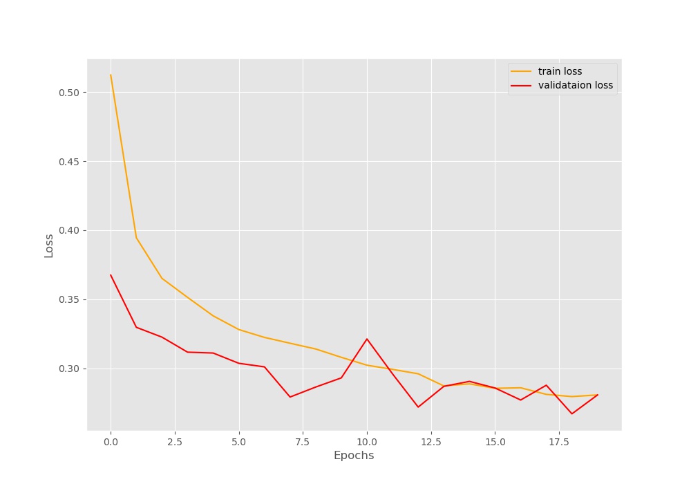
From the above loss plot, we can see that the training loss is decreasing pretty smoothly till the end of 20 epochs. But the validation loss plot is fluctuating a lot. It seems that training any longer than 20 epochs will lead to overfitting. Currently, we are not using any early stopping methods or learning rate scheduler to keep things simple. If we ever want to train further, then we will have to employ those as well. As of now, we have a training and validation loss of 0.2807 after training.

These numbers are alright, but we won’t know how well our model is actually performing until we test it on unseen images. That is what we will be doing in the next section.

Writing the Test Code to Test Our Trained Model on Unseen Fashion Images

We will write our test code in this section. As we already have our trained model weights, this section is going to be very simple.

All of this code will into the test.py Python file.

The Argument Parser and Loading the Trained Model

We will create a simple argument parser using which we will provide the input image path. The following code block contains all the imports, the argument parser, loading the trained model weights, and defining the image transforms as well.

import torch
import cv2
import torchvision.transforms as transforms
import numpy as np
import joblib
import argparse

from models import MultiHeadResNet50

parser = argparse.ArgumentParser()
parser.add_argument('-i', '--input', required=True, help='path to input image')
args = vars(parser.parse_args())

# define the computation device
device = torch.device('cuda' if torch.cuda.is_available() else 'cpu')

model = MultiHeadResNet50(pretrained=False, requires_grad=False)
checkpoint = torch.load('../outputs/model.pth')
model.load_state_dict(checkpoint['model_state_dict'])
model.to(device)
model.eval()

transform = transforms.Compose([
    transforms.ToPILImage(),
    transforms.Resize((224, 224)),
    transforms.ToTensor(),
    transforms.Normalize(mean=[0.485, 0.456, 0.406],
                         std=[0.229, 0.224, 0.225])
])

For the image tranforms, we are resizing the image to 224×224 dimension, converting them tensor, and applying the ImageNet normalization.

Read the Image and Forward Pass Through the Model

We will read the image from the argument parser path. After certain preparation steps, we will forward pass the image through the model.

# read an image
image = cv2.imread(args['input'])
# keep a copy of the original image for OpenCV functions
orig_image = image.copy()
image = cv2.cvtColor(image, cv2.COLOR_BGR2RGB)
# apply image transforms
image = transform(image)
# add batch dimension
image = image.unsqueeze(0).to(device)

# forward pass the image through the model
outputs = model(image)
# extract the three output
output1, output2, output3 = outputs
# get the index positions of the highest label score
out_label_1 = np.argmax(output1.detach().cpu())
out_label_2 = np.argmax(output2.detach().cpu())
out_label_3 = np.argmax(output3.detach().cpu())

At line 33, we are keeping an original copy of the image that we can use for OpenCV functions. Then we are converting the color space to RGB, applying the transforms, and adding a batch dimension as well.

At line 41, we feed the image to the model ang get three outputs that we extract at line 43. From lines 45 to 47, we get the labels by mapping the highest value output to its index position.

Get the Label Names and Show the Image with Multiple Lables

The following are the few final steps that we need to do to get the results.

Let’s write the code first, then we will go for the explnantion.

# load the label dictionaries
num_list_gender = joblib.load('../input/num_list_gender.pkl')
num_list_master = joblib.load('../input/num_list_master.pkl')
num_list_sub = joblib.load('../input/num_list_sub.pkl')

# get the keys and values of each label dictionary
gender_keys = list(num_list_gender.keys())
gender_values = list(num_list_gender.values())
master_keys = list(num_list_master.keys())
master_values = list(num_list_master.values())
sub_keys = list(num_list_sub.keys())
sub_values = list(num_list_sub.values())

final_labels = []
# append the labels by mapping the index position to the values 
final_labels.append(gender_keys[gender_values.index(out_label_1)])
final_labels.append(master_keys[master_values.index(out_label_2)])
final_labels.append(sub_keys[sub_values.index(out_label_3)])

# write the label texts on the image
cv2.putText(
    orig_image, final_labels[0], (10, 25), cv2.FONT_HERSHEY_SIMPLEX, 
    0.8, (0, 255, 0), 2, cv2.LINE_AA 
)
cv2.putText(
    orig_image, final_labels[1], (10, 50), cv2.FONT_HERSHEY_SIMPLEX, 
    0.8, (0, 255, 0), 2, cv2.LINE_AA 
)
cv2.putText(
    orig_image, final_labels[2], (10, 75), cv2.FONT_HERSHEY_SIMPLEX, 
    0.8, (0, 255, 0), 2, cv2.LINE_AA 
)

# visualize and save the image
cv2.imshow('Predicted labels', orig_image)
cv2.waitKey(0)
save_name = args['input'].split('/')[-1]
cv2.imwrite(f"../outputs/{save_name}", orig_image)

• First, we load the dictionaries that we had saved as pickled files to the disk. These contain the category names to label mapping.
• Starting from line 54 to 59, we get the keys as well as the values for each of the three labels. Using these we can easily get the category names by providing the index position of the category values.
• We map the index position of the values to the category names from line 63 to 65. This gives us all the three category names that our model has predicted. And we append those to the final_labels list.
• After that we use cv2.putText() function to write the category names on the images.
• Finally, we show the image on the screen and save the result to disk as well.

This completes writing our testing code as well. Now we can test our model on new and unseen images.

Execute test.py to Test on New Images

We have a few images inside the test folder. Let’s try some of them.

python test.py --input ../input/test_data/image_2.jpg

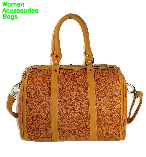
Our model is categorizing the purse into three categories. For the gender, it is predicting women, for the masterCategory, it is predicting accessories, and for the subCategory, it is predicting bags. In my opinion, the results are pretty good. They seem legit and not just randomly guessed.

Moving on to the next image.

python test.py --input ../input/test_data/image_3.jpg

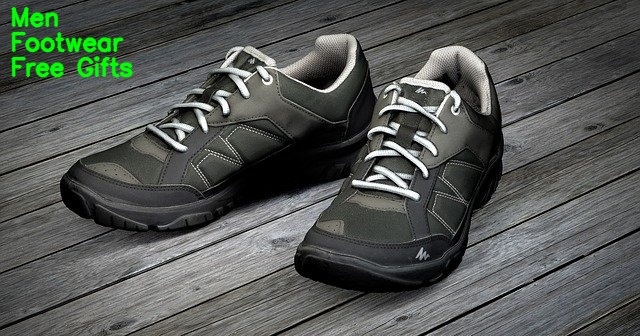
For the shoes, our model seems to be making some mistakes. The first two predictions, men and footwear seem perfectly correct. But for some reason, the model is predicting the third label as free gifts. Here, shoes would have been a much apt prediction.

One final image to test our model.

python test.py --input ../input/test_data/image_4.jpg

Our model is again predicting all the three labels correctly. For the ring, the three predictions are women, accessories, and jewellery. I don’t think that the predictions can be any more correct from this.

As of now our model is predicting the categories pretty well. Obviously, more training will help as we saw in the case of the shoe. Also, we have not utilized all the labels fields present in the dataset’s CSV file. Using those and expanding the project would be a great idea.

Summary and Conclusion

In this tutorial, you got to learn how to customize a pre-trained ResNet50 neural network into a multi-head image classifier. Using the custom deep learning model, we classified fashion item images into multiple categories. I hope that you got to learn something new from this tutorial.

If you have any doubts, thoughts, or suggestions, then please leave them in the comment section. I will surely address them.

You can contact me using the Contact section. You can also find me on LinkedIn, and Twitter.