Adam Optimizer for Deep Learning Optimization

In this tutorial, you will learn how to set up small experimentation and compare the Adam optimizer and the SGD optimizer (Stochastic Gradient Descent) optimizers for deep learning optimization. Specifically, you will learn how to use Adam for deep learning optimization.

For a successful deep learning project, the optimization algorithm plays a crucial role. Stochastic Gradient Descent (I will refer to it as SGD from here on) has played a major role in many successful deep learning projects and research experiments.

But SGD has its own limitations as well. The requirement of excessive tuning of the hyperparameters is one of them. Recently the Adam optimization algorithm has gained a lot of popularity. Adam was developed by Diederik P. Kingma, Jimmy Ba in 2014 and works well in place of SGD. But that does not mean SGD is not used in the industry anymore. It has its benefits and uses. Still in this tutorial, we will focus on the Adam optimization algorithm and its benefits.

About the Adam Optimizer

In this section, we will briefly go over the benefits of the Adam optimizer. Then we will move on to the implementation and coding part where you will have hands-on experience comparing Adam and SGD over the CIFAR10 dataset.

As per the authors of the paper, the name Adam is derived from adaptive moment estimation.

Quoting the authors from the papers:

The method is straightforward to implement, is computationally efficient has little memory requirements, is invariant to diagonal rescaling of the gradients, and is well suited for problems that are large in terms of data and/or parameters.

ADAM: A METHOD FOR STOCHASTIC OPTIMIZATION

The above are some of the reasons why Adam can be the first choice for deep learning optimization.

Benefits of Adam Optimization

Let’s briefly go over the benefits of Adam in this section.

Adaptive Learning Rate

The most beneficial nature of Adam optimization is its adaptive learning rate. As per the authors, it can compute adaptive learning rates for different parameters.

This is in contrast to the SGD algorithm. SGD maintains a single learning rate throughout the network learning process. We can always change the learning rate using a scheduler whenever learning plateaus. But we need to do that through manual coding.

The method computes individual adaptive learning rates for
different parameters from estimates of first and second moments of the gradients…

ADAM: A METHOD FOR STOCHASTIC OPTIMIZATION

The adaptive learning rate feature is one of the biggest reasons why Adam works across a number of models and datasets.

Combine the Benefits of RMSProp and AdaGrad

AdaGrad (Duchi et al., 2011) works well with sparse gradients while the network learns. And RMSProp (Tieleman & Hinton, 2012) works well in on-line non-stationary settings.

Adam optimizer combines the benefits of the AdaGrad and RMSProp at the same time. This means that it does not require a stationary objective and works with sparse gradients as well.

Adam Works Well in Case of Noisy Objectives

Data subsampling can lead to noisy objectives. Implementing dropout regularization can also lead to noisy objectives in deep neural network training. In such cases, we need efficient stochastic optimization techniques.

Adam works well in such cases of stochastic objectives with high-dimensional parameter spaces.

Some Other Benefits

There are some other benefits that make Adam an even better optimizer. Most of the following points are directly referred to from the paper.

• It is straightforward to implement without much tuning.
• Adam is computationally efficient.
• It is memory efficient and has little memory requirements.
• Adam works well in cases in large datasets and large parameter settings.

Now, let’s go over some of the results of the Adam optimization from the paper itself.

Interested to know how SGD with Warm Restarts works? Then don’t miss out on the article Stochastic Gradient Descent with Warm Restarts.

Results of Using the Adam Algorithm for Deep Learning Optimization

I have taken these results directly from the Experiments section (section 6) of the original paper.

Going over the results will give us a better idea of how much better is the Adam algorithm for deep learning optimization and neural network training.

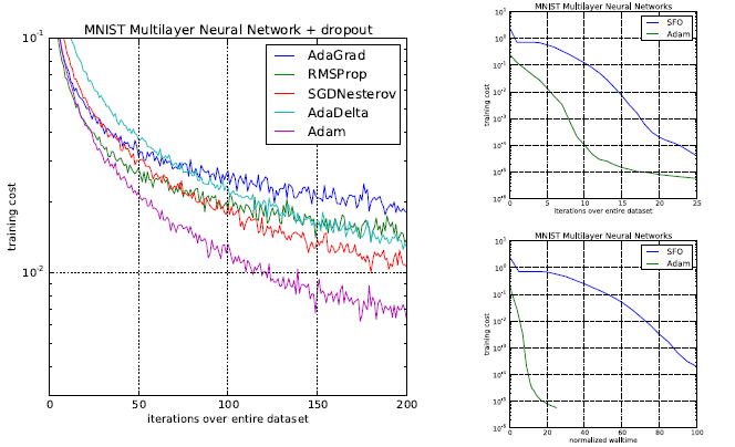
Figure 1 shows the results when using Adam for training a multilayer neural network. The training is done on the very popular MNIST dataset. The training takes place for 200 epochs. And we can see that the Adam algorithm surpasses all the other optimization techniques. Not only it converges faster, but also the cost is much lower than the other optimization techniques.

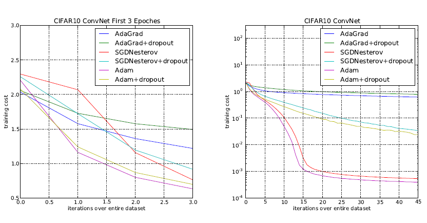
Figure 2 shows the results when using a convolutional neural network for training on the CIFAR10 dataset. In this case also, the Adam optimizer surpasses all the other optimization techniques. Although SGD with Nesterov momentum is close, still Adam has a lower cost and faster convergence.

This shows that Adam can be a good choice for many problems in neural network training.

We will end the theoretical discussion about Adam optimizer here. Note that we did not cover the mathematical details here. If you want to get into the details and learn more about the algorithm, you should give the paper a read.

In the next section, we will discuss the practical (coding) aspects of this tutorial.

Comparing Adam Optimizer and SGD Optimizer

We will try to replicate some of the results from the paper further on in this tutorial. We will compare the Adam optimizer to the SGD optimizer. And obviously, we will write the code for the same. The following are the details of the implementation.

• The dataset: We will use the CIFAR10 dataset in our coding.
• SGD optimizer: We will use the SGD optimizer with Nesterov momentum.
• The neural network: We will use the convolutional neural network architecture with dropout as described in the paper. We will go over the details while writing the neural network code.
• Comparison: We will compare the training and validation loss plots for both Adam and SGD optimizers.

Also, we will use the PyTorch deep learning framework in this tutorial. So, go ahead and install it if you do not have it already.

We will try to keep the code as modular as possible. This will ensure that you can expand this little experimentation into a project later on. Maybe you will want to add more neural network architectures for comparison or even add larger datasets for training. For a good experimentation procedure, we will need a good project directory structure. We will go over that in the next section.

The Project Directory Structure

The following is the project directory structure for this tutorial.

├───input
│   └───data
│       ├───cifar-10-batches-py
├───outputs
└───src
│    adam_vs_sgd.py
│    model.py
│    plot.py
│    run.sh

• The input folder has a data subfolder. This data folder will contain the CIFAR10 dataset that we will download using the torchvision dataset module.
• outputs folder will contain all the training and other outputs that our python code will produce. This also includes the training and validation loss plots.
• The src folder contains 4 files.
  • adam_vs_sgd.py python script will contain the code to train and compare the Adam and SGD optimizers on the CIFAR10 dataset.
  • model.py will contain the neural network architecture.
  • run.sh will contain the commands to train the neural network using Adam and SGD optimizers. We will go over the details while writing the code.
  • Finally, we will use the plot.py python script to plot the training and validation loss line graphs.

This is all the preparation we need. Now, we can move over to writing the code for comparing Adam and SGD optimizers on the CIFAR10 dataset.

Building the Convolutional Neural Network Architecture

In this section, we will write the code to build the convolutional neural network architecture that we will use for training. We will follow the same design as in the paper.

The code in this section will go inside the model.py file inside the src folder.

The Imports and Modules

The following are the imports and modules that we will need along the way.

import torch
import torch.nn as nn
import torch.nn.functional as F

This is all we need to build our CNN model.

The CNN Module

The next block of code defines the complete CNN architecture that we will use. We name our model CNN().

class CNN(nn.Module):
    def __init__(self):
        super(CNN, self).__init__()
        self.conv1 = nn.Conv2d(in_channels=3, out_channels=64, kernel_size=5, padding=1)
        self.conv2 = nn.Conv2d(in_channels=64, out_channels=64, kernel_size=5, padding=1)
        self.conv3 = nn.Conv2d(in_channels=64, out_channels=128, kernel_size=5, padding=1)
        self.pool = nn.MaxPool2d(3, 2)
        self.dropout = nn.Dropout2d(0.5)
        self.fc1 = nn.Linear(in_features=128, out_features=1000)
        self.fc2 = nn.Linear(in_features=1000, out_features=10)

    def forward(self, x):
        x = F.relu(self.conv1(x))
        x = self.dropout(x)
        x = self.pool(x)
        x = F.relu(self.conv2(x))
        x = self.pool(x)
        x = F.relu(self.conv3(x))
        x = self.pool(x)
        # get the batch size and reshape
        bs, _, _, _ = x.shape
        x = F.adaptive_avg_pool2d(x, 1).reshape(bs, -1)
        x = F.relu(self.fc1(x))
        x = self.dropout(x)
        out = self.fc2(x)
        return out

In the __init__() function, first we define the different CNN layers.

• First, we have three convolutional layers with 64, 64, and 128 output channels respectively.
• Then we define a Max-Pooling layer with a size of 3×3 and a stride of 2.
• We also define a dropout layer with a probability of 0.5
• Then we have two fully connected linear layers. The first linear layer has 1000 output features. The second linear layer has 10 output features that correspond to the 10 classes of the CIFAR10 dataset.

Then coming to the forward() function. This follows all the norms that are given in the paper.

• We apply the ReLU activation function to every layer except for the last linear layer.
• As per the paper, we apply dropout after the input layer and the first fully connected layer.

You will see that the network is pretty simple. We need to compare Adam and SGD optimizers here. So, we follow what the authors did in their original experiments.

Python Code to Compare Adam Optimizer and SGD Optimizer

All the code in this section will go into the adam_vs_sgd.py file inside the src folder. So, go ahead and create an empty python script.

Let’s start with all the imports and modules that we will need along the way.

from torchvision import datasets
from torch.utils.data import DataLoader
from tqdm import tqdm

import numpy as np
import torch
import matplotlib
import matplotlib.pyplot as plt
import torchvision.transforms as transforms
import argparse
import model
import torch.optim as optim
import torch.nn as nn
import joblib

The above block of code imports all the libraries and modules that we need for writing the code.

We will define an argument parser for parsing the command line arguments. We will give our choice of the optimizer as an argument while executing the python file.

# construct the argument parser and parse the arguments
parser = argparse.ArgumentParser()
parser.add_argument('-o', '--optimizer', help='the optimizer to use for training', 
                    default='adam', choices=['adam', 'sgd'])
args = vars(parser.parse_args())

The choice of the optimizer is either the Adam optimizer or the SGD optimizer.

Next, we will define some learning parameters that will mostly stay constant throughout the learning process.

# learning parameters
batch_size = 128
epochs = 45
lr = 0.001
device = torch.device('cuda' if torch.cuda.is_available() else 'cpu')

In the above code block:

• At line 2, we have a batch size of 128 (as per the paper).
• We will train the neural network for 45 epochs.
• The learning rate (line 4) is 0.001.
• Finally, on line 5, we define the computation device (CPU or GPU).

Define the Training and Validation Transforms

Here, we will define the training and validation transforms for the CIFAR10 dataset. In PyTorch, generally transforming the dataset means converting the dataset into tensors and normalizing them. In addition to that, we can apply some image preprocessing steps as well.

The authors applied whitening to the pixels in the original experiments. But PyTorch does not provide any direct way to carry whitening transforms. Therefore, we will apply some other transformations to the image. This is an important step. Applying some sort of transforms and preprocessing steps to the images will make the neural network see variations of the image that are in the dataset. This can prevent overfitting.

# define transforms
transform_train = transforms.Compose([
            transforms.RandomCrop(32, padding=4),
            transforms.RandomHorizontalFlip(),
            transforms.ToTensor(),
            transforms.Normalize((0.4914, 0.4822, 0.4465), (0.2023, 0.1994, 0.2010)),
        ])

transform_val = transforms.Compose([
    transforms.ToTensor(),
    transforms.Normalize((0.4914, 0.4822, 0.4465), (0.2023, 0.1994, 0.2010)),
])

We have two transforms in the code block, transform_train and transform_val.

• We will apply transform_train to the training dataset. Also, We randomly crop the images and randomly flip the images horizontally. Then convert the images to tensors and apply the normalization.
• For the transform_val, we only convert the validation data to tensors and normalize the values.

Prepare the Training and Validation Set

Now, we will prepare the training and validation datasets. We can easily get the CIFAR10 data using torchvision’s datasets module.

If the data is not already present, then it will download into input/data folder. First, let’s prepare the training and validation data.

# train and validation data
train_data = datasets.CIFAR10(
    root='../input/data',
    train=True,
    download=True,
    transform=transform_train
)
val_data = datasets.CIFAR10(
    root='../input/data',
    train=False,
    download=True,
    transform=transform_val
)

We apply the transform_train and transform_val to the training and validation data respectively.

Next, we will prepare the training and validation data loaders.

# training and validation data loaders
train_loader = DataLoader(
    train_data,
    batch_size=batch_size,
    shuffle=True
)
val_loader = DataLoader(
    val_data,
    batch_size=batch_size,
    shuffle=False
)

We use the 128 batch size for both, train_loader and val_loader.

Initialize the Model, Optimizer, and Loss Function

We have already imported the model.py file into the adam_vs_sgd.py file. Now, we just need to initialize the model and load it onto the computation device.

model = model.CNN().to(device)

Note that using a GPU for training will be much faster than using a CPU.

Now, we will define the optimizer. Remember that the user can give the optimizer of choice as either Adam or SGD. So, we will create a dictionary and name it optimizer_group. This dictionary will contain both the optimizer and the values. The following code will make things clear.

optimizer_group = {
    'adam': [optim.Adam(model.parameters(), lr=lr, betas=(0.9, 0.999), eps=1e-8, weight_decay=0.0005)], 
    'sgd': [optim.SGD(model.parameters(), lr=lr, nesterov=True, momentum=0.9)]    
}
optimizer = optimizer_group[args['optimizer']][0]

The dictionary has two keys. One is 'adam' and the other one is 'sgd'. The values are Adam and SGD optimizers which we define as lists. For the Adam optimizer, we have provided all the default values explicitly. We also apply the L2 weight decay with a rate of 0.0005. For the SGD optimizer, as per the paper, we apply the Nesterov momentum with a value of 0.9.

At line 5, we initialize the optimizer. First, we get the optimizer key from the command line argument. Then we know that the first value in the key-value pair is the optimizer definition. So, we just get hold of the first value in the list. Using such a dictionary, we can define as many optimizers as we want, if we ever want to carry on with the project even further.

Finally, we need to define the loss function. For that, we will use the CrossEntropyLoss function.

criterion = nn.CrossEntropyLoss()

Define the Training Function

Here, we will define the training function that will train the neural network on the training data. If you have worked with PyTorch before, then you will find it very easy to understand. There is nothing fancy here. We will call the training function as fit().

# training function
def fit(model, dataloader):
    print('Training')
    model.train()
    train_running_loss = 0.0
    train_running_correct = 0
    for i, data in tqdm(enumerate(dataloader), total=int(len(train_data)/dataloader.batch_size)):
        data, target = data[0].to(device), data[1].to(device)
        optimizer.zero_grad()
        outputs = model(data)
        loss = criterion(outputs, target)
        train_running_loss += loss.item()
        _, preds = torch.max(outputs.data, 1)
        train_running_correct += (preds == target).sum().item()
        loss.backward()
        optimizer.step()
        
    train_loss = train_running_loss/len(dataloader.dataset)
    train_accuracy = 100. * train_running_correct/len(dataloader.dataset)    
    return train_loss, train_accuracy

First, we get the model into training mode using model.train(). Then we define train_running_loss and train_running_correct to keep track of batch-wise loss and accuracy. As usual, we iterate through the train data loader from line 7. We calculate the loss, and the accuracy, backpropagate the gradients and update the parameters. Finally, we return train_loss and train_accuracy for each epoch at line 20.

The Validation Function

We do not need to backpropagate the gradients or update the parameters while validating. We also will get the model into evaluation mode using model.eval(). And everything will be within the with torch.no_grad() block.

#validation function
def validate(model, dataloader):
    print('Validating')
    model.eval()
    val_running_loss = 0.0
    val_running_correct = 0
    with torch.no_grad():
        for i, data in tqdm(enumerate(dataloader), total=int(len(val_data)/dataloader.batch_size)):
            data, target = data[0].to(device), data[1].to(device)
            outputs = model(data)
            loss = criterion(outputs, target)
            
            val_running_loss += loss.item()
            _, preds = torch.max(outputs.data, 1)
            val_running_correct += (preds == target).sum().item()
        
        val_loss = val_running_loss/len(dataloader.dataset)
        val_accuracy = 100. * val_running_correct/len(dataloader.dataset)        
        return val_loss, val_accuracy

Training and Validating

We will train and validate the model for 45 epochs.

print(f"Training with {args['optimizer']}")
train_loss , train_accuracy = [], []
val_loss , val_accuracy = [], []
for epoch in range(epochs):
    print(f"Epoch {epoch+1} of {epochs}")
    train_epoch_loss, train_epoch_accuracy = fit(model, train_loader)
    val_epoch_loss, val_epoch_accuracy = validate(model, val_loader)
    train_loss.append(train_epoch_loss)
    train_accuracy.append(train_epoch_accuracy)
    val_loss.append(val_epoch_loss)
    val_accuracy.append(val_epoch_accuracy)
    print(f"Train Loss: {train_epoch_loss:.4f}, Train Acc: {train_epoch_accuracy:.2f}")
    print(f'Val Loss: {val_epoch_loss:.4f}, Val Acc: {val_epoch_accuracy:.2f}')

We will append each epoch’s training loss and accuracy to train_loss and train_accuracy lists respectively. Similarly for validation loss and validation accuracy.

After the training completes, we will not plot the loss line graphs in this file. Instead, we will save the train_loss , train_accuracy, val_loss, and val_accuracy as .pkl files to the disk. Then we will load those in the plot.py file and plot the graphs in that file. This will help us to plot the line graphs for different optimizers on the same plot.

The following block of code saves those values as .pkl files to the outputs folder.

joblib.dump(train_loss, f"../outputs/train_loss_{args['optimizer']}.pkl")
joblib.dump(val_loss, f"../outputs/val_loss_{args['optimizer']}.pkl")
joblib.dump(train_accuracy, f"../outputs/train_accuracy_{args['optimizer']}.pkl")
joblib.dump(val_accuracy, f"../outputs/val_accuracy_{args['optimizer']}.pkl")

This marks the end of our training code. Now we need to execute the adam_vs_sgd.py file.

Executing adam_vs_sgd.py Using run.sh File

We will not directly execute the adam_vs_sgd.py file from the command line. Remember that we need to execute the file twice, once with adam argument and then again with sgd argument. We can do that easily with the command line as there are only two choices. But what if we also want to expand the project for other optimizers, add more deep learning models, or add more datasets? Then we will have to keep on getting back to the command line every time we need to execute the file.

Instead, we can create a shell script (a .sh file) and add all the execution commands to the file just once. Then we need to execute that script only and all the training with all the different parameters and arguments will take one after the other.

Now, go ahead and create a run.sh file inside the src folder. After that add the following two commands to the file.

python adam_vs_sgd.py --optimizer adam

python adam_vs_sgd.py --optimizer sgd

The two lines are the python commands that we would have executed in the terminal. Instead, we add those to the shell script. You can add many more such commands and then just execute the script. This will execute all the commands one by one.

Now, get onto your terminal. Go to your project folder and then navigate to the src folder in the terminal. To execute, just type the following command.

sh run.sh

The python file will execute with the two command line arguments one after the other. The following is the truncated output.

Training with adam
Epoch 1 of 45
Training
391it [00:22, 17.53it/s]
Validating
79it [00:02, 39.39it/s]
Train Loss: 0.0141, Train Acc: 33.68
Val Loss: 0.0116, Val Acc: 45.79
...
Training with sgd
Epoch 1 of 45
Training
391it [00:15, 24.49it/s]
Validating
79it [00:02, 34.65it/s]
Train Loss: 0.0172, Train Acc: 16.76
Val Loss: 0.0156, Val Acc: 27.84
Epoch 2 of 45
...
Epoch 45 of 45
Training
391it [00:15, 25.04it/s]
Validating
79it [00:02, 34.08it/s]
Train Loss: 0.0068, Train Acc: 70.34
Val Loss: 0.0056, Val Acc: 75.82

Plotting the Loss Line Graphs

All the training loss, training accuracy, and validation loss, validation accuracy lists are saved to the disk as .pkl files.

Go ahead and create a plot.py file inside the src folder.

After that add the following imports to the python file.

import joblib
import matplotlib.pyplot as plt

We just need the joblib and matplotlib libraries.

Next, we will write the code to plot the training loss line graphs for both the Adam and the SGD optimizer.

# loss plot
train_loss_adam = joblib.load('../outputs/train_loss_adam.pkl')
train_loss_sgd = joblib.load('../outputs/train_loss_sgd.pkl')
plt.plot(train_loss_adam, color='green', label='Adam')
plt.plot(train_loss_sgd, color='blue', label='SGDNesterov')
plt.xlabel('Epochs')
plt.ylabel('Train Loss')
plt.legend()
plt.savefig(f"../outputs/train_loss.png")
plt.show()

At lines 2 and 3, we load the train loss lists for the Adam and SGD optimizers. Then we plot and save the line graphs to the outputs folder on the disk.

We will do the same for the validation loss list files.

val_loss_adam = joblib.load('../outputs/val_loss_adam.pkl')
val_loss_sgd = joblib.load('../outputs/val_loss_sgd.pkl')
plt.plot(val_loss_adam, color='purple', label='Adam')
plt.plot(val_loss_sgd, color='orange', label='SGDNesterov')
plt.xlabel('Epochs')
plt.ylabel('Validation Loss')
plt.legend()
plt.savefig(f"../outputs/val_loss.png")
plt.show()

We save the validation loss graphs to the disk as well.

Analyzing the Loss Plots

In this section, we will analyze the loss plots that we have saved to the disk.

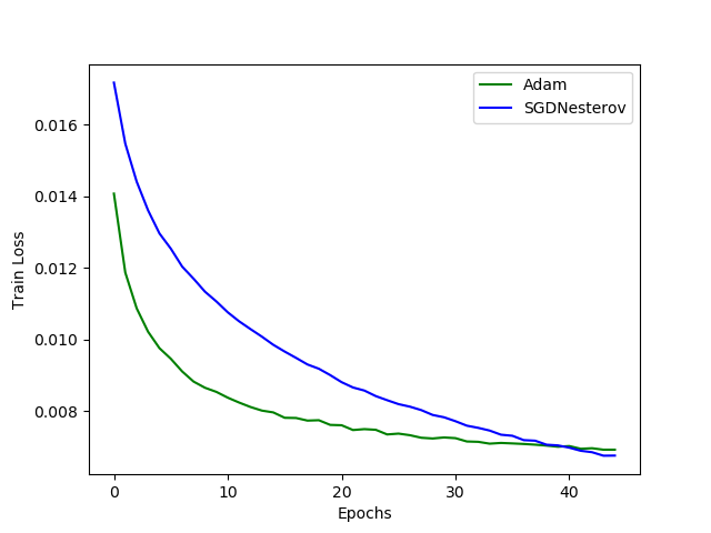
Figure 3 shows the train loss line graphs for the Adam and SGD optimizers. We can see that the Adam optimizer converges much faster. In fact, its loss is consistently less than SGD from the beginning till epoch number 40. After 40 epochs, SGD seems to have less loss value than the Adam optimizer.

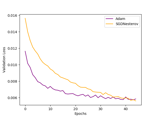
Figure 4 shows the validation loss graphs. In this case, also, the convergence of Adam is much faster than SGD. It has lower loss values than SGD to 40 epochs after which SGD has less loss than Adam.

From the above analysis we can conclude the following:

• Using the Adam optimizer will lead to much faster convergence.
• It can have low cost or loss values from the beginning compared to other optimizers.
• Adam optimizer is consistent across training and validation sets.
• SGD, although slower, will converge in the end. But this may be because of Nesterov momentum as well.
• SGD may need much more hyperparameter tuning for good convergence when compared to Adam.
• Whereas Adam works very well with the default hyperparameters. This may be because of its adaptive learning rate property.

Now, you can go ahead and expand the project with more optimizer comparisons, neural network models, and datasets as well.

Summary and Conclusion

In this tutorial, you learned about the Adam optimizer. You also got to know the benefits of Adam optimizer compared to other optimizers.

You also got hands-on experience in comparing the Adam and SGD optimizers while training a neural network on the CIFAR10 dataset.

If you have any doubts, thoughts, or suggestions, then use the comment section. I will surely address them.

You can contact me using the Contact section. You can also find me on LinkedIn, and Twitter.