An Introduction to k-Nearest Neighbors in Machine Learning

In machine learning, there are many traditional algorithms that will remain relevant for a long time. k-Nearest Neighbor (KNN) is one such algorithm that we will get to know in this article. KNN is a simple and efficient algorithm. It is easy to understand the methodology of KNN as well. In this article, we will cover an introduction to k-Nearest Neighbors in machine learning.

k-Nearest Neighbor Technique

You can use the k-nearest neighbor algorithm for both classification and regression. Also, KNN can be used for both supervised and unsupervised learning.

The method used in KNN is fairly simple. Suppose that we have a dataset containing N examples. Now, in KNN, there is no learning technique. When we implement KNN on the N samples, it simply remembers the data points.

To remember all the data points, KNN stores all the data in memory. This can prove to be a problem for larger datasets.

After storing all the data into memory, suppose we give the k-nearest neighbor algorithm a new data to classify. As it has all the training data in memory, it will simply compare the new data with k of its nearest data points. And that’s the reason it is called the k-nearest neighbor technique.

By now, you must have guessed that larger datasets can be very costly when trying to implement the nearest neighbor algorithm.

As the model is not learned, we also call KNN a non-parametric algorithm. This means that it does not make any assumptions about the training data. For this reason, KNN works well for classification problems.

Choosing K in KNN

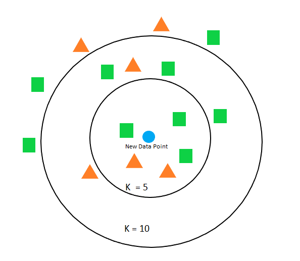
When using KNN, to classify a new data point, we need to specify K. K is the most important hyperparameter in the KNN algorithm. KNN makes predictions based on the K nearest instances in the training data.

It is better to start with a small K value and increase the value gradually. With a smaller K value, the algorithms will form a smaller decision boundary. It will also go over less number of instances for comparison. In most cases, we need to find a large and optimal value of K which can form a large decision boundary.

Choosing K is always a question of bias-variance tradeoff. When K is small, it will lead to low bias but higher variance and vice-versa for larger K value.

Instead of checking K values randomly, we can also use k-fold cross-validation.

Algorithms in KNN

In KNN, all of the training data is stored in memory. When we have a new data point we need to find the nearest neighbors for that data point. For this reason, we need fast and optimized data structures where the search can be as fast as possible.

In KNN, we have three major such implementations for storing all of the data. They are:

Brute force approach: This is the most basic approach. Using brute force involves computing distances between all pairs of data points in the dataset. Suppose we have \(N\) samples with \(D\) dimensions. The search complexity is \(O[DN^{2}]\). For this reason, the brute force approach works well for small datasets. But for large datasets, the search time can be a lot more.

K-D tree: KD tree is a tree-based data structure that helps overcome the computational cost of the brute force approach.

KD tree greatly helps in reducing the number of distance calculations. The nearest neighbor search complexity for KD tree is \(O[D N \log(N)]\). This is much less than the brute force approach when we consider larger datasets. KD tree stands for K-Dimensional tree. So, the KD tree can become inefficient as well when the number of dimensions \(D\) becomes very large.

Ball Tree: Ball tree helps to overcome the inefficiencies of the KD tree for higher dimensions. Ball tree is much faster for storing multidimensional data. Ball tree partitions data in nested hyperspheres called balls. In ball tree, each node contains a hypersphere. And each hypersphere contains a subset of points which are needed to be searched.

Problems in KNN

KNN works best when the dataset is not too large. The main reason being that the whole dataset is stored in memory. Therefore, when the number of samples increases, then KNN can become inefficient. This is especially true when applying the brute force approach.

Another thing to notice is that KNN models are not really ‘trained‘. The dataset is just memorized. So, with large datasets, the main problem begins when finding the neighbors for a new data point, that is the testing phase. Suppose that we want to classify a new point using KNN, then for really large datasets, KNN will become computationally expensive for finding the neighbors.

Even if we use the KD tree technique, then large dimensionality can be another problem. In this case, the computation mostly depends on D (the number of dimensions). So, with more dimensions, the search time also increases. This is otherwise known as the curse of dimensionality in machine learning.

More on KNN Approaches

If you want to gain further knowledge on the algorithms used in KNN, then you can refer the following articles:
– Ball Tree Wikipedia.
– KD Tree Wikipedia.
– Scikit-Learn Nearest Neighbor Docs.

Summary and Conclusion

I hope that you learned new things about KNN from this article. This article is a short theoretical introduction to KNN. You can leave your thoughts in the comment section and I will try to address them. You can also find me on LinkedIn, and Twitter.