Training VGG11 from Scratch using PyTorch

In this tutorial, we will be training the VGG11 deep learning model from scratch using PyTorch.

Last week we learned how to implement the VGG11 deep neural network model from scratch using PyTorch. We went through the model architectures from the paper in brief. We saw the model configurations, different convolutional and linear layers, and the usage of max-pooling and dropout as well. And then we wrote the VGG11 neural network architecture from scratch.

This week, we will use the architecture from last week (VGG11) and train it from scratch. This will give us a good idea of how building and training a model on our own from scratch feels like.

• Last week (part one): Implementing VGG11 from scratch using PyTorch.
• This week (part two): Training our implemented VGG11 model from scratch using PyTorch
• Next week (part three): Implementing all the VGG models in a generalized manner using the PyTorch deep learning framework.

So, what are we going to cover in this tutorial?

• Going over the dataset and directory structure.
  • We will train our VGG11 from scratch using the Digit MNIST dataset.
• Getting into the coding part.
  • Preparing the dataset.
  • Training and validating the model.
  • We will also follow the same optimizer settings as mentioned in the original VGG paper.
  • We will also see class-wise accuracy for each of the digit classes while validating with each epoch.
• Analyzing the loss and accuracy plots after training.
• Testing the trained model on digit images (which are not part of the MNIST dataset).

Let us get into the depth of the tutorial now and get into training VGG11 from scratch using PyTorch.

The Directory Structure, Dataset, and PyTorch Version

In this section, we will go over the dataset that we will use for training, the project directory structure, and the PyTorch version.

The Dataset

For training, we will use the Digit MNIST dataset. Why the Digit MNIST dataset? It is a simple dataset, it is small, and the model will very likely converge in a few epochs even when training from scratch.

Our main goal is to learn how writing a model architecture on our own and training from scratch affects accuracy and loss. And how good the model can become. We can surely look at bigger and more complex datasets in future posts. In the original paper, the authors trained the VGG models on the ImageNet dataset. We surely cannot do that here as that requires a lot of computational power and training time as well.

Also, we can load the MNIST dataset using the torchvision.dataset module. This makes the work of procuring the dataset a bit easier.

The Directory Structure

We will follow the below directory structure for this project. It will be easier for you to follow along if you use the same structure as well.

├── input
│   └── test_data
│       ├── eight.jpg
│       ├── two.jpg
│       └── zero.jpg
├── outputs
│   ├── accuracy.jpg
│   └── loss.jpg
|   ...
├── src
│   ├── data
│   │   └── MNIST
│   ...
│   ├── models.py
│   ├── test.py
│   └── train.py

• The src folder contains the three Python files that we will need in this tutorial. We will get into the details of these shortly.
• The outputs folder will hold the loss and accuracy plots along with the trained VGG11 model.
• Finally input folder contains the test images that we will test our trained model on. The image names and the digits they contain are the same so that we can easily differentiate between them.

You can download the source code and the test data for this tutorial by clicking on the button below.

The PyTorch Version

In this tutorial, we will use PyTorch version 1.8.0. I insist that you install this version, or whatever the latest is when you are reading this. Be sure to use an Anaconda or Python virtual environment to install the latest version. This will ensure that there are no conflicts with other versions and projects.

You can visit the official PyTorch page to install the latest version of PyTorch. Follow the instructions according to your operating system and environment and choose the right version.

There a few other requirements like Matplotlib for saving graph plots and OpenCV for reading images. If you do not have those, feel free to install them as you proceed.

Training VGG11 from Scratch using PyTorch

Let us start with the coding part of this tutorial.

We will begin with the code for the VGG11 model. Then we will move on to write the training script. And finally, we will write the test script which will test our trained model on the test images in the input folder.

Note: The training of the VGG11 model from scratch might take a lot of time depending on the hardware one has. If you do not have a GPU in your own system, then you can run it on Colab Notebook as well. Please click on the button below where you will get access to a pre-set-up Colab notebook with all the code available and ready to run.

The VGG11 Deep Learning Model for Training VGG11 from Scratch using PyTorch

In this section, we will write the code for the VGG11 deep learning model.

Please note that we will not go through a detailed explanation of the architecture here. The previous article discusses the architecture in much detail. You can go through that article if you feel necessary to learn about the details of the VGG11 model.

Now, we can start with the coding of the VGG11 model. All the code here will go into the models.py Python file.

The following block of code contains the whole VGG11 network. This ensures that the code is perfectly readable and indentations are also maintained.

import torch.nn as nn

# the VGG11 architecture
class VGG11(nn.Module):
    def __init__(self, in_channels, num_classes=1000):
        super(VGG11, self).__init__()
        self.in_channels = in_channels
        self.num_classes = num_classes
        # convolutional layers 
        self.conv_layers = nn.Sequential(
            nn.Conv2d(self.in_channels, 64, kernel_size=3, padding=1),
            nn.ReLU(),
            nn.MaxPool2d(kernel_size=2, stride=2),
            nn.Conv2d(64, 128, kernel_size=3, padding=1),
            nn.ReLU(),
            nn.MaxPool2d(kernel_size=2, stride=2),
            nn.Conv2d(128, 256, kernel_size=3, padding=1),
            nn.ReLU(),
            nn.Conv2d(256, 256, kernel_size=3, padding=1),
            nn.ReLU(),
            nn.MaxPool2d(kernel_size=2, stride=2),
            nn.Conv2d(256, 512, kernel_size=3, padding=1),
            nn.ReLU(),
            nn.Conv2d(512, 512, kernel_size=3, padding=1),
            nn.ReLU(),
            nn.MaxPool2d(kernel_size=2, stride=2),
            nn.Conv2d(512, 512, kernel_size=3, padding=1),
            nn.ReLU(),
            nn.Conv2d(512, 512, kernel_size=3, padding=1),
            nn.ReLU(),
            nn.MaxPool2d(kernel_size=2, stride=2)
        )
        # fully connected linear layers
        self.linear_layers = nn.Sequential(
            nn.Linear(in_features=512*7*7, out_features=4096),
            nn.ReLU(),
            nn.Dropout2d(0.5),
            nn.Linear(in_features=4096, out_features=4096),
            nn.ReLU(),
            nn.Dropout2d(0.5),
            nn.Linear(in_features=4096, out_features=self.num_classes)
        )

    def forward(self, x):
        x = self.conv_layers(x)
        # flatten to prepare for the fully connected layers
        x = x.view(x.size(0), -1)
        x = self.linear_layers(x)
        return x

We only need one module for writing the model code, that is the torch.nn module. Now, there are a few things to note here.

• In the __init__() method, we have the in_channels parameter which we will need to pass as an argument when we initialize the model. As we will be using the Digit MNIST dataset, this value will be 1 as all the images are in grayscale format.
• Another parameter is num_classes which defines the output classes in the dataset. This is 1000 by default which corresponds to the 1000 classes of the ImageNet dataset. But Digit MNIST has only 10 classes. So, we will be changing this value as well while initializing the model.
• As the number of neurons is reducing in a few of the layers (like from 1000 to 10 for the output classes), our model will not have 132,863,336 parameters anymore. It will be close to 129 million. We will get to see the exact number when we start the training part.

The above are some of the details that we should keep in mind for the VGG11 model in this tutorial.

This is all we need for the VGG11 model code. Let us now move in to the training script.

The Training Script

We will try to keep the training script as simple as possible. If you have trained any neural network model on the Digit MNIST dataset before, then you will not have any issues in this part.

We will write the training code in the train.py Python script.

The following are all the modules and libraries we need for the training script.

import torch
import torchvision
import torchvision.transforms as transforms
import matplotlib.pyplot as plt
import matplotlib
import torch.nn as nn
import torch.optim as optim

from tqdm import tqdm
from models import VGG11

matplotlib.style.use('ggplot')

Along with all the standard modules that we need, we are also importing our own VGG11 model.

The next block of code defines some of the training configurations. This includes the computation device, the number of epochs to train for, and the batch size.

device = torch.device('cuda' if torch.cuda.is_available() else 'cpu')
print(f"[INFO]: Computation device: {device}")
epochs = 10
batch_size = 32

If you are training on you own system, then it is a lot better if you have a CUDA enabled Nvidia GPU. That will make the training a lot faster.

We will be training the model for 10 epochs with a batch size of 32.

If you face OOM (Out Of Memory) error while training, then reduce the batch size to either 16, or 8, or 4, whichever fits your GPU memory size.

The Image Transforms

The following are the training and validation transforms that we will use.

# our transforms will differ a bit from the VGG paper
# as we are using the MNIST dataset, so, we will directly resize...
# ... the images to 224x224 and not crop them and we will not use...
# ... any random flippings also
train_transform = transforms.Compose(
    [transforms.Resize((224, 224)),
     transforms.ToTensor(),
     transforms.Normalize(mean=(0.5), std=(0.5))])
valid_transform = transforms.Compose(
    [transforms.Resize((224, 224)),
     transforms.ToTensor(),
     transforms.Normalize(mean=(0.5), std=(0.5))])

• In the original paper, the authors used a few augmentations along with the transforms. They used random horizontal flips for augmentations as they were training on the ImageNet dataset. But we are not using any flipping as the dataset is the Digit MNIST. Flipping of digit images can change the property and meaning of the digits.
• We are also directly resizing the images to 224×224 dimensions and are not using any cropping of the pixels. Cropping might also lead to the loss of features in the digit images.
• Other than that, we are converting all the pixels to image tensors and normalizing the pixel values as well.

Datasets and Data Loaders

The next step is to prepare the training and validation datasets and data loaders.

The following block of code does that.

# training dataset and data loader
train_dataset = torchvision.datasets.MNIST(root='./data', train=True,
                                             download=True, 
                                             transform=train_transform)
train_dataloader = torch.utils.data.DataLoader(train_dataset, 
                                               batch_size=batch_size,
                                               shuffle=True)
# validation dataset and dataloader
valid_dataset = torchvision.datasets.MNIST(root='./data', train=False,
                                           download=True, 
                                           transform=valid_transform)
valid_dataloader = torch.utils.data.DataLoader(valid_dataset, 
                                             batch_size=batch_size,
                                             shuffle=False)

We using the torchvision.datasets module to load the MNIST dataset and apply the image transforms. Then we are preparing the data loaders with the batch size that we define above. We are only shuffling the training data loaders and not the validation data loaders.

Initialize the Model, Loss Function, and Optimizer

Here, we will initialize the model, the loss function, and the optimizer.

# instantiate the model
model = VGG11(in_channels=1, num_classes=10).to(device)
# total parameters and trainable parameters
total_params = sum(p.numel() for p in model.parameters())
print(f"[INFO]: {total_params:,} total parameters.")
total_trainable_params = sum(
    p.numel() for p in model.parameters() if p.requires_grad)
print(f"[INFO]: {total_trainable_params:,} trainable parameters.")

# the loss function
criterion = nn.CrossEntropyLoss()
# the optimizer
optimizer = optim.SGD(model.parameters(), lr=0.01, momentum=0.9, 
                      weight_decay=0.0005)

• Notice that the value for in_channels argument is 1 as we are training on the MNIST dataset which has grayscale images. Similarly, num_classes is 10 as the dataset has 10 classes (one for each digit from 0 to 9). Then we are printing the number of parameters of the model.
• We are using the Cross Entropy loss function. The optimizer is SGD just as described in the paper with learning rate of 0.01, momentum of 0.9, and weight decay of 0.0005.

The Training Function

The training function is going to be very simple. Just as any other MNIST training function (or any image classification training function) in PyTorch.

# training
def train(model, trainloader, optimizer, criterion):
    model.train()
    print('Training')
    train_running_loss = 0.0
    train_running_correct = 0
    counter = 0
    for i, data in tqdm(enumerate(trainloader), total=len(trainloader)):
        counter += 1

        image, labels = data
        image = image.to(device)
        labels = labels.to(device)

        optimizer.zero_grad()
        # forward pass
        outputs = model(image)
        # calculate the loss
        loss = criterion(outputs, labels)
        train_running_loss += loss.item()
        # calculate the accuracy
        _, preds = torch.max(outputs.data, 1)
        train_running_correct += (preds == labels).sum().item()
        loss.backward()
        optimizer.step()
    
    epoch_loss = train_running_loss / counter
    epoch_acc = 100. * (train_running_correct / len(trainloader.dataset))
    return epoch_loss, epoch_acc

The training function is very much self-explanatory.

• We are iterating through the training data loader and extracting the labels and images from it.
• Then we are loading the images and labels onto the computation device.
• After that we are forward propagating the images through the model, calculating the loss and the accuracy values. Then we are backpropagating the current loss.
• Finally, we are returning the loss and accuracy for the current epoch.

The Validation Function

The validation function is going to be a little different this time. For each epoch, we will calculate the loss and accuracy as usual. Also, we will calculate the accuracy for each class to get an idea how our model is performing with each epoch.

Let us write the code for the validation function.

# validation
def validate(model, testloader, criterion):
    model.eval()
    
    # we need two lists to keep track of class-wise accuracy
    class_correct = list(0. for i in range(10))
    class_total = list(0. for i in range(10))

    print('Validation')
    valid_running_loss = 0.0
    valid_running_correct = 0
    counter = 0
    with torch.no_grad():
        for i, data in tqdm(enumerate(testloader), total=len(testloader)):
            counter += 1
            
            image, labels = data
            image = image.to(device)
            labels = labels.to(device)

            # forward pass
            outputs = model(image)
            # calculate the loss
            loss = criterion(outputs, labels)
            valid_running_loss += loss.item()
            # calculate the accuracy
            _, preds = torch.max(outputs.data, 1)
            valid_running_correct += (preds == labels).sum().item()

            # calculate the accuracy for each class
            correct  = (preds == labels).squeeze()
            for i in range(len(preds)):
                label = labels[i]
                class_correct[label] += correct[i].item()
                class_total[label] += 1
        
    epoch_loss = valid_running_loss / counter
    epoch_acc = 100. * (valid_running_correct / len(testloader.dataset))

    # print the accuracy for each class after evey epoch
    # the values should increase as the training goes on
    print('\n')
    for i in range(10):
        print(f"Accuracy of digit {i}: {100*class_correct[i]/class_total[i]}")

    return epoch_loss, epoch_acc

• First, we are putting the model into evaluation mode at line 88.
• At lines 90 and 91, we are creating two lists, class_correct and class_total. We need these to keep track of class-wise accuracy for each of the digit classes.
• From line 94 to line 113, it is the general validation code for the dataset. We are not backpropagating the loss for the validation epochs and the code is within the with torch.no_grad() block. This ensures that the gradients are not calculated.
• Starting from line 116, we are writing the code for calculating accuracy for each class.
• For each of the classes in one iteration, we are storing the total correctly predicted labels and the total number of labels in class_correct and class_total lists.
• We are printing the class-wise accuracy at line 129.
• Then we return the epoch-wise loss and accuracy at line 131.

The Training Loop

We will train the model for 10 epochs and will do that using a simple for loop.

# start the training
# lists to keep track of losses and accuracies
train_loss, valid_loss = [], []
train_acc, valid_acc = [], []
for epoch in range(epochs):
    print(f"[INFO]: Epoch {epoch+1} of {epochs}")

    train_epoch_loss, train_epoch_acc = train(model, train_dataloader, 
                                              optimizer, criterion)
    valid_epoch_loss, valid_epoch_acc = validate(model, valid_dataloader,  
                                                 criterion)
    train_loss.append(train_epoch_loss)
    valid_loss.append(valid_epoch_loss)
    train_acc.append(train_epoch_acc)
    valid_acc.append(valid_epoch_acc)

    print('\n')
    print(f"Training loss: {train_epoch_loss:.3f}, training acc: {train_epoch_acc:.3f}")
    print(f"Validation loss: {valid_epoch_loss:.3f}, validation acc: {valid_epoch_acc:.3f}")

    print('-'*50)

• We will store the training & validation losses and accuracies in the train_loss, valid_loss train_acc, and valid_acc lists respectively.
• After each epoch, we are printing the training and loss metrics also.

The final steps are to save the trained model and the accuracy and loss plots to disk.

# save the trained model to disk
torch.save({
            'epoch': epochs,
            'model_state_dict': model.state_dict(),
            'optimizer_state_dict': optimizer.state_dict(),
            'loss': criterion,
            }, '../outputs/model.pth')

# accuracy plots
plt.figure(figsize=(10, 7))
plt.plot(
    train_acc, color='green', linestyle='-', 
    label='train accuracy'
)
plt.plot(
    valid_acc, color='blue', linestyle='-', 
    label='validataion accuracy'
)
plt.xlabel('Epochs')
plt.ylabel('Accuracy')
plt.legend()
plt.savefig('../outputs/accuracy.jpg')
plt.show()
# loss plots
plt.figure(figsize=(10, 7))
plt.plot(
    train_loss, color='orange', linestyle='-', 
    label='train loss'
)
plt.plot(
    valid_loss, color='red', linestyle='-', 
    label='validataion loss'
)
plt.xlabel('Epochs')
plt.ylabel('Loss')
plt.legend()
plt.savefig('../outputs/loss.jpg')
plt.show()
 
print('TRAINING COMPLETE')

We are saving the trained model, the loss plot, and the accuracy inside the outputs folder.

Later on, we will use the trained model to run inference (test) on a few digit images that are inside the input/test_data folder.

Executing train.py for Training the VGG11 Model on the MNIST Dataset

Now, it is time to execute the train.py script and see how our model learns and performs.

Open up your command line/terminal and cd into the src folder inside the project directory. Then type the following command.

python train.py 

You should see output similar to the following.

[INFO]: Computation device: cuda
[INFO]: 128,806,154 total parameters.
[INFO]: 128,806,154 trainable parameters.
[INFO]: Epoch 1 of 10
Training
100%|████████████████████████████████████████████████████████████| 1875/1875 [12:20<00:00,  2.53it/s]
Validation
100%|██████████████████████████████████████████████████████████████| 313/313 [00:42<00:00,  7.32it/s]


Accuracy of digit 0: 0.0
Accuracy of digit 1: 100.0
Accuracy of digit 2: 0.0
Accuracy of digit 3: 0.0
Accuracy of digit 4: 0.0
Accuracy of digit 5: 0.0
Accuracy of digit 6: 0.0
Accuracy of digit 7: 0.0
Accuracy of digit 8: 0.0
Accuracy of digit 9: 0.0
...
[INFO]: Epoch 10 of 10
Training
100%|████████████████████████████████████████████████████████████| 1875/1875 [12:17<00:00,  2.54it/s]
Validation
100%|██████████████████████████████████████████████████████████████| 313/313 [00:43<00:00,  7.25it/s]


Accuracy of digit 0: 99.79591836734694
Accuracy of digit 1: 99.73568281938326
Accuracy of digit 2: 99.70930232558139
Accuracy of digit 3: 99.5049504950495
Accuracy of digit 4: 99.28716904276986
Accuracy of digit 5: 98.4304932735426
Accuracy of digit 6: 98.95615866388309
Accuracy of digit 7: 98.15175097276264
Accuracy of digit 8: 99.79466119096509
Accuracy of digit 9: 98.41427155599604


Training loss: 0.021, training acc: 99.333
Validation loss: 0.024, validation acc: 99.190
--------------------------------------------------
TRAINING COMPLETE

In the above block, I have only shown the outputs from the first and last epoch. We can observe how after the first epoch, the model did not learn almost anything. The class-wise accuracy of each digit except digit 1 is 0.

But by the last epoch, our VGG11 model was able to achieve 99.190 validation accuracy and 0.024 validation loss. That is really good.

Let us take a look at the accuracy and loss plots to get some more ideas.

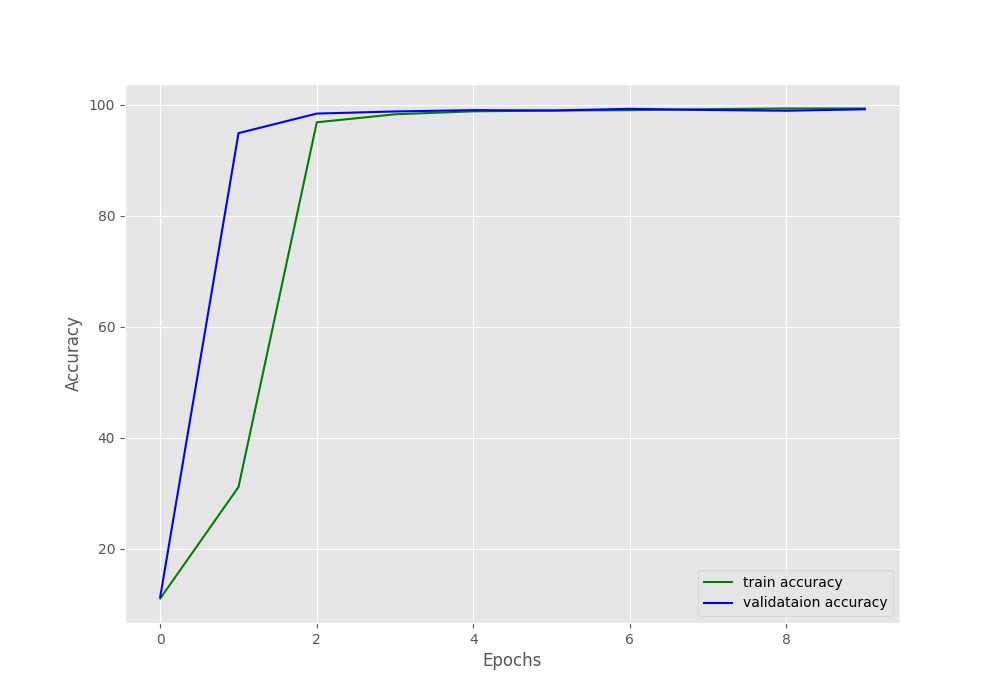
The learning of the model in terms of accuracy just shot up by epoch 2. After that, the learning was very gradual till epoch 6 and improved very little by the last epoch. This tells that for VGG11, Digit MNIST model is not a very difficult one to learn.

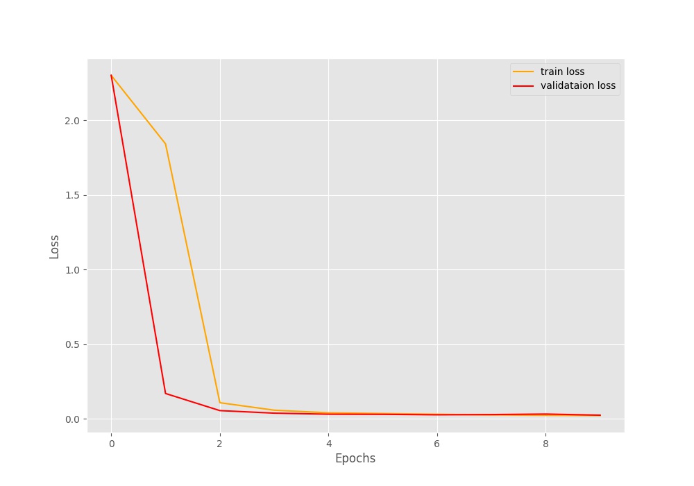
We can see a similar trend with the loss values also. It decreased by a large amount by second epoch and then it was very gradual.

One thing to note here. Although, the loss and accuracy values improved very gradually after a few epochs, still, they are were improving. Would training for more epochs help, or would it lead to overfitting? I hope that you explore this proposition and let everyone know in the comment section.

Testing the Trained VGG11 Model on Unseen Images

We used the training and validation data for the learning of the model. This means that we cannot use the validation data anymore for inference on the trained model.

For this, we will test our trained VGG11 model on a few unseen digit images.

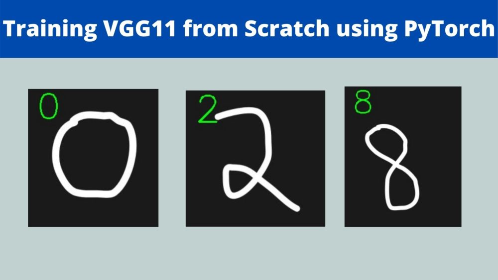
Figure 4 shows images of three digits we will use for testing the trained VGG11 model.

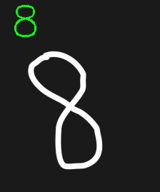
We have digits 2, 0, and 8. You will find these images inside the input/test_data folder if you have downloaded the source code and data for this tutorial. You are free to use your own dataset as well.

Let us start writing the code for the test script. This code will go inside the test.py Python script.

Test Script for Inference

The following are the libraries and modules that we will need for the test script.

import torch
import cv2
import glob as glob
import torchvision.transforms as transforms
import numpy as np

from models import VGG11

• We have the cv2 module to read the images.
• glob module will help us get all the test images’ paths.
• And we surely need the VGG11 module to initialize the VGG11 model.

Load the Trained Weights and Define the Transforms

The next step is to initialize the trained model and load the trained weights. We will also define the test transforms.

# inferencing on CPU
device = 'cpu'
# initialize the VGG11 model
model = VGG11(in_channels=1, num_classes=10)
# load the model checkpoint
checkpoint = torch.load('../outputs/model.pth')
# load the trained weights
model.load_state_dict(checkpoint['model_state_dict'])
model.to(device)
model.eval()

# simple image transforms
transform = transforms.Compose([
    transforms.ToPILImage(),
    transforms.Resize((224, 224)),
    transforms.ToTensor(),
    transforms.Normalize(mean=[0.5],
                         std=[0.5])
])

Note that we are inferencing on the CPU and not the GPU. For testing a few images, this should do just fine. From line 11, we are initializing the model, loading the checkpoint, and trained weights, moving the model to the computation device, and getting the model into evaluation mode.

Then we are defining the transforms which will resize the images, convert them to tensor, and normalize them as well.

Reading the Images and Passing them Through the Model

We have three images in total. We will just loop over their paths, read, pre-process, and forward propagate them through the model.

# get all the test images path
image_paths = glob.glob('../input/test_data/*.jpg')

for i, image_path in enumerate(image_paths):
    orig_img = cv2.imread(image_path)
    # convert to grayscale to make the image single channel
    image = cv2.cvtColor(orig_img, cv2.COLOR_BGR2GRAY)
    image = transform(image)
    # add one extra batch dimension
    image = image.unsqueeze(0).to(device)
    # forward pass the image through the model
    outputs = model(image)
    # get the index of the highest score
    # the highest scoring indicates the label for the Digit MNIST dataset
    label = np.array(outputs.detach()).argmax()
    print(f"{image_path.split('/')[-1].split('.')[0]}: {label}")
    # put the predicted label on the original image
    cv2.putText(orig_img, str(label), (15, 50), cv2.FONT_HERSHEY_SIMPLEX, 
                2, (0, 255, 0), 2)
    # show and save the resutls
    cv2.imshow('Result', orig_img)
    cv2.waitKey(0)
    cv2.imwrite(f"../outputs/result_{i}.jpg", orig_img)

• At line 28, we are capturing all the test images’ paths using the glob module.
• Then we start to loop over the image paths. First, we read the image and convert them to grayscale to make them single color channel images.
• We then transform the images, add an extra batch dimension so that their shape becomes [1, 1, 224, 224], which the model expects.
• At line 38, we forward propagate the image through the model.
• At line 41, we get the highest scoring index position from the outputs tensor. For the MNIST dataset, the highest scoring index will be the predicted label.
• Then we print the image name and the predicted label. This is just for some extra information on the terminal.
• Finally, we put the predicted label text on the original image frame, show the result on screen, and save the results to disk as well.

This completes our testing script as well.

Running test.py for Testing the VGG11 model

From within the src folder, type the following command on the command line/terminal.

python test.py 

You should see the following output.

two: 2
zero: 0
eight: 8

And the following figure shows all the digits with the predicted labels.

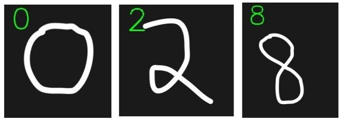
Our VGG11 model is predicting all the digit images correctly.

From here on, if you want to take this small project a bit further, you may try a few more things.

• Train for some more epochs.
• Train with a different learning rate.
• Try out the Adam optimizer.
• Test the model on more complex digit images.

If you carry the above experiments, then try posting your findings in the comment section for other to know as well.

Summary and Conclusion

In this tutorial, we trained a VGG11 deep neural network model from scratch on the Digit MNIST dataset. We started with initializing the model, training the model, and observed the accuracy and loss plots as well. After that, we also tested our model on unseen digit images to see how it performs. I hope that you learned something new from this article.

If you have any doubts, thoughts, or suggestions, then please leave them in the comment section. I will surely address them.

You can contact me using the Contact section. You can also find me on LinkedIn, and Twitter.