Training ResNet18 from Scratch using PyTorch

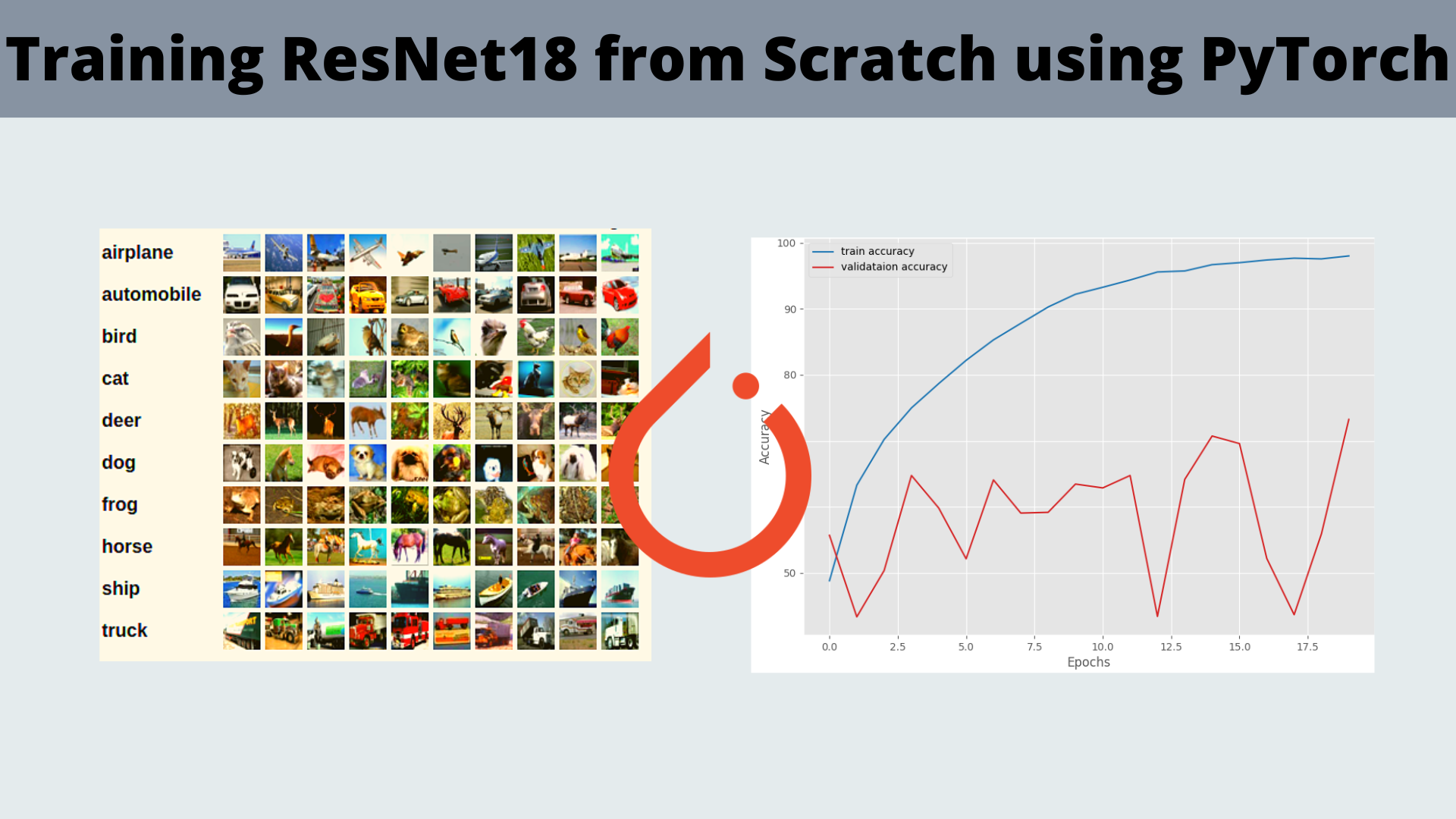
In this blog post, we will be training a ResNet18 model from scratch using PyTorch. We will be using a model that we have we have written from scratch as covered in the last tutorial.

In the last blog post, we replicated the ResNet18 neural network model from scratch using PyTorch. That led us to discover how to:

• Write the Basic Blocks of the ResNets.
• Create the identity connections that ResNets are famous for.
• And how to combine everything to create the final ResNet18 module.

In this post, we will take it a bit further. Only creating a model is not enough. We need to verify whether it is working (able to train) properly or not.

For that reason, we will train it on a simple dataset. And to check that indeed it is doing its job, we will also train the Torchvision ResNet18 model on the same dataset. The technical details will follow in the next sections.

For now, let’s check out all the points that we will cover in this post:

• We will start with exploring the dataset. We will use the CIFAR10 dataset to train the ResNet18 models in this post.
• Then we will move over to the discussion of the project’s directory structure.
• Next, we will move to the training section which will include:
  • The code for the ResNet18 model creation that we already covered in the last post.
  • The training and validation functions.
  • Preparation of the datasets.
  • And the training of the models.

Let’s get into the details without any further delay.

The CIFAR10 Dataset

Anyone who has been in the field of deep learning for a while is not new to the famous CIFAR10 dataset.

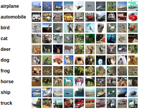
The CIFAR10 dataset contains 60000 RGB images each of size 32×32 in dimension.

Out of the 60000 images, 50000 are for training and the rest 10000 for testing/validation.

All the images in the CIFAR10 dataset belong to one of the following 10 classes:

• airplane
• automobile
• bird
• cat
• deer
• dog
• frog
• horse
• ship
• truck

CIFAR10 is a good dataset to test out any custom model. If it is able to achieve high accuracy on this dataset, then it is probably correct and will train on other datasets as well.

If you wish to explore the dataset more, please visit the official website.

Directory Structure

The following is the directory structure for the project containing all the files and subdirectories.

.
├── data
│   ├── cifar-10-batches-py
│   │   ├── batches.meta
│   │   ├── data_batch_1
│   │   ├── data_batch_2
│   │   ├── data_batch_3
│   │   ├── data_batch_4
│   │   ├── data_batch_5
│   │   ├── readme.html
│   │   └── test_batch
│   └── cifar-10-python.tar.gz
├── outputs
│   ├── resnet_scratch_accuracy.png
│   ├── resnet_scratch_loss.png
│   ├── resnet_torchvision_accuracy.png
│   └── resnet_torchvision_loss.png
├── resnet18.py
├── resnet18_torchvision.py
├── train.py
├── training_utils.py
└── utils.py

• The data directory contains the CIFAR10 dataset that we will download from Torchvision.
• The outputs directory contains the accuracy and loss plots for both the training experiments, ResNet18 built from scratch, and the Torchvision ResNet18 as well.
• Directly inside the project directory, we have five Python code files. We will get into the details of these in their respective sections

When downloading the zip file for this tutorial, you will get access to all the Python files and output plots. After extracting the file, it will already be in the above directory structure. You can run any training experiment you want.

PyTorch Version

The code for this blog post uses PyTorch version 1.12.0 and Torchvision version 0.13.0.

Be sure to install this or the latest available version before moving ahead.

You can install PyTorch from the official website.

Training ResNet18 from Scratch using PyTorch

Let’s get into the coding parts of the blog post now.

Download Code

For the most part, we will only have a brief overview of all the Python files except for the training script.

The Utility Scripts

Let’s start with the utility scripts. All the code here will go into the utils.py file. This Python file contains the function definitions to load the training and validation dataset, and also the function definition to save the accuracy & loss plots.

The following code block contains the import statements and the function definition to load the dataset.

import matplotlib.pyplot as plt
import os

from torch.utils.data import DataLoader
from torchvision import datasets
from torchvision.transforms import ToTensor

plt.style.use('ggplot')

def get_data(batch_size=64):
    # CIFAR10 training dataset.
    dataset_train = datasets.CIFAR10(
        root='data',
        train=True,
        download=True,
        transform=ToTensor(),
    )

    # CIFAR10 validation dataset.
    dataset_valid = datasets.CIFAR10(
        root='data',
        train=False,
        download=True,
        transform=ToTensor(),
    )

    # Create data loaders.
    train_loader = DataLoader(
        dataset_train, 
        batch_size=batch_size,
        shuffle=True
    )
    valid_loader = DataLoader(
        dataset_valid, 
        batch_size=batch_size,
        shuffle=False
    )
    return train_loader, valid_loader

The get_data() function prepares the training and validation sets and the data loaders as well. Next is the code for saving the training and loss plots.

def save_plots(train_acc, valid_acc, train_loss, valid_loss, name=None):
    """
    Function to save the loss and accuracy plots to disk.
    """
    # Accuracy plots.
    plt.figure(figsize=(10, 7))
    plt.plot(
        train_acc, color='tab:blue', linestyle='-', 
        label='train accuracy'
    )
    plt.plot(
        valid_acc, color='tab:red', linestyle='-', 
        label='validataion accuracy'
    )
    plt.xlabel('Epochs')
    plt.ylabel('Accuracy')
    plt.legend()
    plt.savefig(os.path.join('outputs', name+'_accuracy.png'))
    
    # Loss plots.
    plt.figure(figsize=(10, 7))
    plt.plot(
        train_loss, color='tab:blue', linestyle='-', 
        label='train loss'
    )
    plt.plot(
        valid_loss, color='tab:red', linestyle='-', 
        label='validataion loss'
    )
    plt.xlabel('Epochs')
    plt.ylabel('Loss')
    plt.legend()
    plt.savefig(os.path.join('outputs', name+'_loss.png'))

The train_acc, valid_acc, train_loss, and valid_loss are lists containing the respective values for each epoch. The name parameter is a string indicating whether the accuracy and loss values are from training the ResNet18 that was built from scratch or from the Torchvision ResNet18 training. This ensures that the plots are saved with different names on to the disk.

Training and Validation Helper Functions for Training ResNet18 from Scratch using PyTorch

Now, we will write the code for the training and validation functions. These are very simple image classification training and validation code. We need not go into the depth of these two functions.

This code will go into the training_utils.py file.

First, is the training function.

import torch

from tqdm import tqdm

# Training function.
def train(model, trainloader, optimizer, criterion, device):
    model.train()
    print('Training')
    train_running_loss = 0.0
    train_running_correct = 0
    counter = 0
    for i, data in tqdm(enumerate(trainloader), total=len(trainloader)):
        counter += 1
        image, labels = data
        image = image.to(device)
        labels = labels.to(device)
        optimizer.zero_grad()
        # Forward pass.
        outputs = model(image)
        # Calculate the loss.
        loss = criterion(outputs, labels)
        train_running_loss += loss.item()
        # Calculate the accuracy.
        _, preds = torch.max(outputs.data, 1)
        train_running_correct += (preds == labels).sum().item()
        # Backpropagation
        loss.backward()
        # Update the weights.
        optimizer.step()
    
    # Loss and accuracy for the complete epoch.
    epoch_loss = train_running_loss / counter
    # epoch_acc = 100. * (train_running_correct / len(trainloader.dataset))
    epoch_acc = 100. * (train_running_correct / len(trainloader.dataset))
    return epoch_loss, epoch_acc

Next is the validation function.

# Validation function.
def validate(model, testloader, criterion, device):
    model.eval()
    print('Validation')
    valid_running_loss = 0.0
    valid_running_correct = 0
    counter = 0

    with torch.no_grad():
        for i, data in tqdm(enumerate(testloader), total=len(testloader)):
            counter += 1
            
            image, labels = data
            image = image.to(device)
            labels = labels.to(device)
            # Forward pass.
            outputs = model(image)
            # Calculate the loss.
            loss = criterion(outputs, labels)
            valid_running_loss += loss.item()
            # Calculate the accuracy.
            _, preds = torch.max(outputs.data, 1)
            valid_running_correct += (preds == labels).sum().item()
        
    # Loss and accuracy for the complete epoch.
    epoch_loss = valid_running_loss / counter
    epoch_acc = 100. * (valid_running_correct / len(testloader.dataset))
    return epoch_loss, epoch_acc

The above two functions will do the heavy lifting for us during the training procedure. We just need to call the functions by passing the appropriate arguments.

The ResNet18 Model Code

As we know, we will be training two different ResNet18 models in this blog post. One of the ResNet18 models that we built from scratch in the last tutorial. And the other one is the Torchvision ResNet18 model.

• If you need to get into the details of building the ResNet18 from scratch using PyTorch, then please visit the previous post. You can also find the same code in the resnet18.py file that you download with this post.
• For the Torchvision ResNet18 model, we need to customize a few things. First of all, we do not want to load any ImageNet pretrained weights. We can take care of that in the training script directly by passing the required arguments. And we also need to change the number of classes from 1000 (ImageNet) to CIFAR10 (10). You can find the required code for the Torchvision ResNet18 model in the resnet18_torchvision.py file.

For now, let’s focus on the executable training script.

The Training Script

This is one of the important parts of the experiment. The training script encapsulates everything that we need to start the training.

All the code shown here will go into the train.py script.

Let’s start by importing the required modules, defining the argument parser, and setting the seed for reproducibility.

import torch
import torch.nn as nn
import torch.optim as optim
import argparse
import numpy as np
import random

from resnet18 import ResNet, BasicBlock
from resnet18_torchvision import build_model
from training_utils import train, validate
from utils import save_plots, get_data

parser = argparse.ArgumentParser()
parser.add_argument(
    '-m', '--model', default='scratch',
    help='choose model built from scratch or the Torchvision model',
    choices=['scratch', 'torchvision']
)
args = vars(parser.parse_args())

# Set seed.
seed = 42
torch.manual_seed(seed)
torch.cuda.manual_seed(seed)
torch.backends.cudnn.deterministic = True
torch.backends.cudnn.benchmark = True
np.random.seed(seed)
random.seed(seed)

In the import statements, we can see:

• We are importing the ResNet class and the BasicBlock class from the custom ResNet18 module.
• And we are also importing the build_model function from the resnet18_torchvision module.

We will need both of these for separate experiments.

For the argument parser, we have only one flag. The --model flag lets us choose between the ResNet18 from scratch model or the torchvision ResNet18 model. We will build the appropriate model based on this command line input.

Starting from lines 22 to 28, we set all the seeds for reproducibility.

Defining the Learning Parameters and Loading the Models

Let’s define all the learning and training parameters. Along with that, we also need to load the model according to the --model input from the command line. The following code block shows that.

# Learning and training parameters.
epochs = 20
batch_size = 64
learning_rate = 0.01
device = torch.device('cuda:0' if torch.cuda.is_available() else 'cpu')

train_loader, valid_loader = get_data(batch_size=batch_size)

# Define model based on the argument parser string.
if args['model'] == 'scratch':
    print('[INFO]: Training ResNet18 built from scratch...')
    model = ResNet(img_channels=3, num_layers=18, block=BasicBlock, num_classes=10).to(device)
    plot_name = 'resnet_scratch'
if args['model'] == 'torchvision':
    print('[INFO]: Training the Torchvision ResNet18 model...')
    model = build_model(pretrained=False, fine_tune=True, num_classes=10).to(device) 
    plot_name = 'resnet_torchvision'
# print(model)

# Total parameters and trainable parameters.
total_params = sum(p.numel() for p in model.parameters())
print(f"{total_params:,} total parameters.")
total_trainable_params = sum(
    p.numel() for p in model.parameters() if p.requires_grad)
print(f"{total_trainable_params:,} training parameters.")

# Optimizer.
optimizer = optim.SGD(model.parameters(), lr=learning_rate)
# Loss function.
criterion = nn.CrossEntropyLoss()

We will train the models for 20 epochs. The batch size for the data loaders is going to be 64. As we will be using the SGD optimizer, so we use a learning rate of 0.01.

On line 35, we load the training and validation data loaders.

Starting from line 38, we load the required ResNet18 model based on the --model flag. If the input is scratch, then we load the ResNet18 model that was built from scratch. You can see that the num_layers to the ResNet class is provided as 18.

If the input is torchvision, then we load the ResNet18 model from Torchvision.

In both cases, we initialize a plot_name string. We will pass down this string while saving the accuracy and loss plots for appropriate naming.

Next, we define the SGD optimizer, and the Cross-Entropy loss function.

The Main Execution Block

Now, coming to the main execution block (if __name__ == '__main__').

if __name__ == '__main__':
    # Lists to keep track of losses and accuracies.
    train_loss, valid_loss = [], []
    train_acc, valid_acc = [], []
    # Start the training.
    for epoch in range(epochs):
        print(f"[INFO]: Epoch {epoch+1} of {epochs}")
        train_epoch_loss, train_epoch_acc = train(
            model, 
            train_loader, 
            optimizer, 
            criterion,
            device
        )
        valid_epoch_loss, valid_epoch_acc = validate(
            model, 
            valid_loader, 
            criterion,
            device
        )
        train_loss.append(train_epoch_loss)
        valid_loss.append(valid_epoch_loss)
        train_acc.append(train_epoch_acc)
        valid_acc.append(valid_epoch_acc)
        print(f"Training loss: {train_epoch_loss:.3f}, training acc: {train_epoch_acc:.3f}")
        print(f"Validation loss: {valid_epoch_loss:.3f}, validation acc: {valid_epoch_acc:.3f}")
        print('-'*50)
        
    # Save the loss and accuracy plots.
    save_plots(
        train_acc, 
        valid_acc, 
        train_loss, 
        valid_loss, 
        name=plot_name
    )
    print('TRAINING COMPLETE')

Here, we have a for loop for training the chosen model. The appropriate accuracies and loss values are stored in their respective lists.

After the training ends, we save the accuracy and loss plots by providing the plot_name argument.

This is all we need for the training script.

ResNet18 from Scratch Training

In this subsection, we will train the ResNet18 that we built from scratch in the last tutorial.

All the code is ready, we just need to execute the train.py script with the --model argument from the project directory.

python train.py --model scratch

The following is the truncated output.

Files already downloaded and verified
Files already downloaded and verified
[INFO]: Training ResNet18 built from scratch...
11,181,642 total parameters.
11,181,642 training parameters.
[INFO]: Epoch 1 of 20
Training
100%|██████████████████████████████████████████████████████████████████| 782/782 [00:14<00:00, 53.26it/s]
Validation
100%|█████████████████████████████████████████████████████████████████| 157/157 [00:01<00:00, 132.54it/s]
Training loss: 1.425, training acc: 48.816
Validation loss: 1.248, validation acc: 55.690
--------------------------------------------------
[INFO]: Epoch 2 of 20
Training
100%|██████████████████████████████████████████████████████████████████| 782/782 [00:09<00:00, 80.23it/s]
Validation
100%|█████████████████████████████████████████████████████████████████| 157/157 [00:01<00:00, 127.43it/s]
Training loss: 1.030, training acc: 63.282
Validation loss: 1.782, validation acc: 43.340
--------------------------------------------------
.
.
.
[INFO]: Epoch 19 of 20
Training
100%|██████████████████████████████████████████████████████████████████| 782/782 [00:09<00:00, 82.34it/s]
Validation
100%|█████████████████████████████████████████████████████████████████| 157/157 [00:01<00:00, 136.07it/s]
Training loss: 0.069, training acc: 97.556
Validation loss: 2.718, validation acc: 55.930
--------------------------------------------------
[INFO]: Epoch 20 of 20
Training
100%|██████████████████████████████████████████████████████████████████| 782/782 [00:09<00:00, 82.25it/s]
Validation
100%|█████████████████████████████████████████████████████████████████| 157/157 [00:01<00:00, 128.54it/s]
Training loss: 0.057, training acc: 98.002
Validation loss: 1.362, validation acc: 73.240
--------------------------------------------------
TRAINING COMPLETE

By the end of 20 epochs, we have a training accuracy of 98% and a validation accuracy of 73.24%. But looking at the graphs will give us more insights.

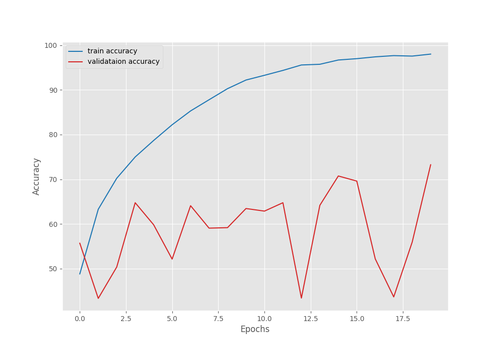
Although the training looks pretty good, we can see a lot of fluctuations in the validation accuracy and loss curves. The CIFAR10 dataset is not the easiest of the datasets. Moreover, we are training from scratch without any pretrained weights. But we will get to actually know whether our ResNet18 model is performing as it should only after training the Torchvision ResNet18 model.

Torchvision ResNet18 Training

Now, let’s train the Torchvision ResNet18 model without using any pretrained weights.

python train.py --model torchvision

The following block shows the outputs.

Files already downloaded and verified
Files already downloaded and verified
[INFO]: Training the Torchvision ResNet18 model...
[INFO]: Not loading pre-trained weights
[INFO]: Fine-tuning all layers...
11,181,642 total parameters.
11,181,642 training parameters.
[INFO]: Epoch 1 of 20
Training
100%|██████████████████████████████████████████████████████████████████| 782/782 [00:11<00:00, 68.90it/s]
Validation
100%|█████████████████████████████████████████████████████████████████| 157/157 [00:01<00:00, 131.75it/s]
Training loss: 1.593, training acc: 42.024
Validation loss: 1.620, validation acc: 42.600
--------------------------------------------------
[INFO]: Epoch 2 of 20
Training
100%|██████████████████████████████████████████████████████████████████| 782/782 [00:09<00:00, 79.97it/s]
Validation
100%|█████████████████████████████████████████████████████████████████| 157/157 [00:01<00:00, 125.95it/s]
Training loss: 1.239, training acc: 55.592
Validation loss: 1.511, validation acc: 47.780
--------------------------------------------------
.
.
.
[INFO]: Epoch 19 of 20
Training
100%|██████████████████████████████████████████████████████████████████| 782/782 [00:09<00:00, 81.92it/s]
Validation
100%|█████████████████████████████████████████████████████████████████| 157/157 [00:01<00:00, 131.04it/s]
Training loss: 0.082, training acc: 97.198
Validation loss: 2.281, validation acc: 59.130
--------------------------------------------------
[INFO]: Epoch 20 of 20
Training
100%|██████████████████████████████████████████████████████████████████| 782/782 [00:09<00:00, 82.07it/s]
Validation
100%|█████████████████████████████████████████████████████████████████| 157/157 [00:01<00:00, 132.05it/s]
Training loss: 0.069, training acc: 97.756
Validation loss: 3.006, validation acc: 51.950
--------------------------------------------------
TRAINING COMPLETE

We have slightly lower training accuracy when using the Torchvision ResNet18 model. Let’s take a look at the plots.

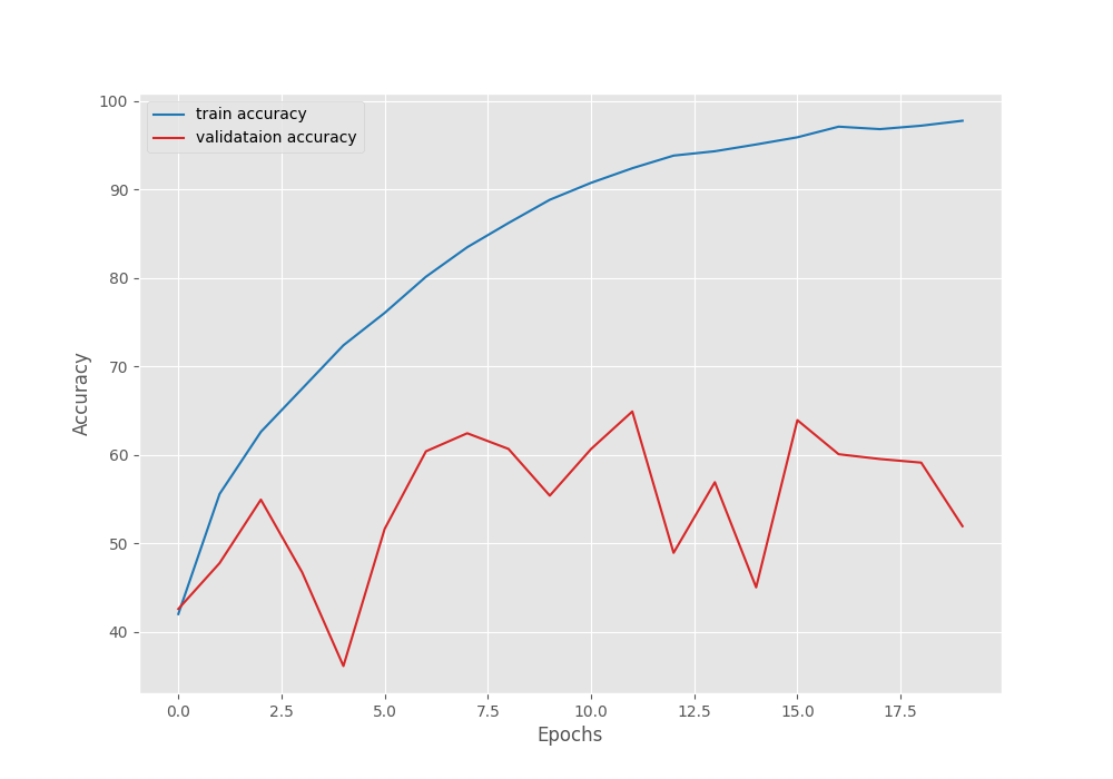
We can see a similar type of fluctuations in the validation curves here as well.

Most of these issues can be solved by using image augmentation and a learning rate scheduler.

But from the above experiments, we can conclude that our ResNet18 model built from scratch is working at least as well as the Torchvision one if not better.

Summary and Conclusion

In this blog post, we carried out the training of a ResNet18 model using PyTorch that we built from scratch. We used the CIFAR10 dataset for this. To compare the results, we also trained the Torchvision ResNet18 model on the same dataset. We found out that the custom ResNet18 model is working well. I hope that this blog post was helpful to you.

If you have any doubts, thoughts, or suggestions, please leave them in the comment section. I will surely address them.

You can contact me using the Contact section. You can also find me on LinkedIn, and Twitter.