

The handwritten digits MNIST data set is good enough to get started with image classification, but it is getting old. Therefore, in this article you will be tackling another variant of the MNIST data set, the Fashion MNIST data set. Doing Fashion MNIST classification with Keras can be a lot of fun for those who are getting started with neural networks and deep learning.
What is the Fashion MNIST Data Set
The Fashion MNIST data set consists of 70000 gray scale images of fashion products. This was proposed by Han Xiao, Kashif Rasul, and Roland Vollgraf as a replacement for the classic hand-written digits data set (read the paper here).
The data set is almost similar to the digits data set. It contains 60000 images for training purpose and 10000 images for testing. It can be just as good a starting point to dive into deep learning with Keras. And that is exactly what we are going to do in this article. Let’s move ahead.
Loading and Analyzing the Data
The Fashion MNIST data comes bundled with Keras. So, we can directly load the data after importing Keras.
import tensorflow as tf
import numpy as np
import matplotlib.pyplot as plt

from tensorflow import keras
fashion_mnist = keras.datasets.fashion_mnist

(X_train, y_train), (X_test, y_test) = fashion_mnist.load_data()
The images are all 28 x 28 Numpy arrays stored as pixel intensities ranging from 0 to 255. Also, the target labels are from 0 to 9 each categorizing one of the 10 following clothing type:
| Label | Class |
| 0 1 2 3 4 5 6 7 8 9 | T-shirt/top Trouser Pullover Dress Coat Sandal Shirt Sneaker Bag Ankle boot |
But there is one catch here. The names are not included anywhere in the data set. We can create a list comprising of these names. This would help with the visualization in the later stages.
names = ['T-shirt/top', 'Trouser', 'Pullover', 'Dress', 'Coat', 'Sandal',
        'Shirt', 'Sneaker', 'Bag', 'Ankle boot']
Now, let us go through the data that we have:
print(X_train.shape)
(60000, 28, 28)
The training data contains 60000 images all of which are 28 x 28 pixels.
print(y_train)
[9 0 0 ... 3 0 5]
The train labels do not contain anything fancy as well. The images are all classified from 0 to 9 based on the fashion type.
The test set also adheres to similar data structure but with 10000 instances instead of 60000.
Scaling and Visualizing
Let’s visualize the second image in the training set:
plt.imshow(X_train[1])
plt.colorbar()
plt.grid(False)
plt.show()
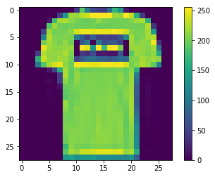
You can see that the pixel intensities range from 0 to 255. We should scale the pixel values so that they range between 0 to 1. But Why? The central idea being neural networks learn much better and faster as well when fed with small, scaled and floating point values.
# Scaling the images
X_train, X_test = X_train / 255.0, X_test / 255.0
Now, visualizing few of the images:
plt.figure(figsize=(16, 12))
for i in range(9):
    plt.subplot(330+i+1)
    plt.xticks([])
    plt.yticks([])
    plt.grid(False)
    plt.imshow(X_train[i])
    plt.xlabel(names[y_train[i]])

plt.colorbar()
plt.show()
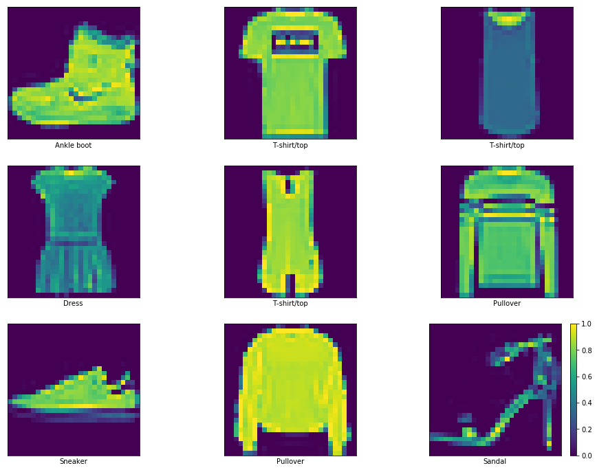
Now you can also see that the pixel intensity values are between 0.0 and 1.0.
Building a Model in Keras
# Stacking up the layers
model = keras.Sequential([
     keras.layers.Flatten(input_shape=(28, 28)),
     keras.layers.Dense(128, activation=tf.nn.relu),
     keras.layers.Dense(10, activation=tf.nn.softmax)
 ])
The code above flattens the 28×28 input_shape to a single vector with 784 values. Two Dense() layers are connected. One is the hidden layer with 128 nodes/neurons and the other is the output layer with 10 neurons. The 10 neurons are for each of the 10 class labels in the data set.
Compiling the Model
# Compiling the model
model.compile(optimizer='adam',
             loss='sparse_categorical_crossentropy',
             metrics=['accuracy'])
In the above block of code, the loss function tells about the accuracy during training. This function is always minimized. The optimizer updates the model based on the loss function and the data. And metrics calculates the accuracy between the training and testing by taking how many images are correctly classified.
Training the Model
model.fit(X_train, y_train, epochs=20)
The training will run for 20 epochs and each epoch will train through the whole data.
Evaluation
accuracy = model.evaluate(X_test, y_test)
print('Accuracy:', accuracy)
10000/10000 [==============================] - 0s 46us/sample - loss: 0.3465 - acc: 0.8885 Accuracy: [0.3464975884974003, 0.8885]
The model gives about 89% accuracy. If you have read my previous article for the MNIST handwritten digits classification with neural networks, then you will know that this accuracy is comparatively less. One reason can be the complexity of the images in the fashion MNIST data. You can always try to improve this accuracy. A good place to start would be augmenting the images. This would give you many new images to train on as well. Be sure to share your results in the comment section if you do so.
Click here to get the code file.
Conclusion
If you liked this article then comment, share and give a thumbs up. If you have any questions or suggestions, just Contact me here. Be sure to subscribe to the website for more content. Follow me on Twitter, LinkedIn, and Facebook to get regular updates.
