With DINOv3 backbones, it has now become easier to train semantic segmentation models with less data and training iterations. Choosing from 10 different backbones, we can find the perfect size for any segmentation task without compromising speed and quality. In this article, we will tackle semantic segmentation with DINOv3. This is a continuation of the DINOv3 series that we started last week.
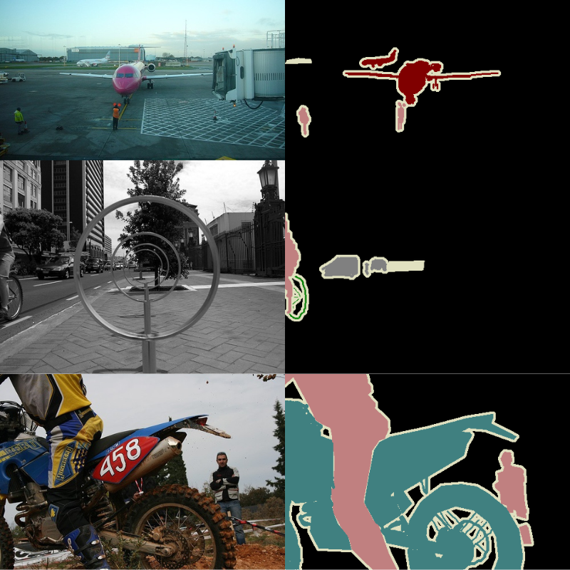
Figure 1. DINOv3 semantic segmentation inference result demo.
Semantic segmentation is a foundational computer vision task. It powers industries such as healthcare, automotive, and sports, among many others. With DINOv3’s range of backbones, we can accelerate the applied research of semantic segmentation for several use cases. The authors of DINOv3 have open sourced the segmentation head pretrained using the 7B backbone. However, using the pretrained 7B parameter model is difficult because of its high VRAM requirements. Therefore, we are going to pretrain our own DINOv3 model for semantic segmentation on the Pascal VOC dataset.
Approach to modeling for semantic segmentation using DINOv3:
Step 1: We will load the pretrained DINOv3 ViT-S/16 backbone.
Step 2: We will add a simple segmentation decoder head on top of the backbone feature extractor.
Step 3: Training the model for semantic segmentation.
What are we going to cover in semantic segmentation with DINOv3?
Discussing the Pascal VOC segmentation dataset.
Discussing the DINOv3 Stack codebase.
Structuring the codebase and configuring files.
Training the DINOv3 model on the VOC segmentation dataset.
Running inference using the trained model.
The Pascal VOC Semantic Segmentation Dataset
We will use the Pascal VOC dataset in this article for training the DINOv3 model. In case you aim to pursue the training of the model, you can download the dataset from the above link.
It contains 1464 training and 1449 validation samples. The segmentation maps are 3-channel RGB masks.
Here are some ground truth samples.
Figure 2. Ground truth samples from the Pascal VOC semantic segmentation dataset.
The dataset contains 21 classes, including the background class.
We will conduct two experiments with the dataset. One is transfer learning while keeping the backbone frozen, and the second one is fine-tuning the entire network.
The following is the dataset directory structure after downloading and extracting it.
The downloaded folder has been renamed to pascal_voc_seg and it contains the voc_2012_segmentation_data subfolder. Inside that, we have the directories for images and masks.
The DINOv3 Stack Codebase
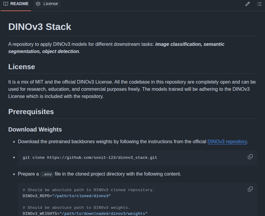
We will use the dinov3_stack GitHub codebase for the segmentation experiments. This is an open-source project that I am maintaining for downstream tasks with DINOv3. Right now, it includes image classification with DINOv3 and semantic segmentation.
Figure 3. DINOv3 Stack GitHub.
Soon, object detection will also be included in the codebase.
The Project Directory Structure
Let’s take a look at the project directory structure.
The input directory contains the dataset that we donwloaded earlier.
The outputs directory will contain all the training and inference results.
We have the semantic segmentation source code inside the src/img_seg directory. The train_segmentation.py is the executable script that starts the training experiment. infer_seg_image.py and infer_seg_video.py contain the source code for running semantic segmentation inference on images and videos.
The segmentation_configs folder contains YAML files with class names of the dataset that we are using. This is for easier configuration and training. We will go through the details in one of the later sections.
The dinov3 folder is the cloned DINOv3 repository that we need for loading the models. Please refer to previous week’s article for more detail.
Finally, the weights folder contain the pretrained DINOv3 ViT-S/16 weights that we need for initializing the backbone.
You do not need to clone the dinov3_stack repository. All the necessary codebase has been provided as a downloadable zip file. The remaining of the setup steps are covered in the following subsections.
Download Code
Setting Up and Dependencies
After downloading the above codebase and extracting it, open a terminal inside the directory.
Then, download the DINOv3 ViT-S/16 pretrained weight by filling out the form by clicking one of the links in the following table.
You should receive an email with links to all the files. The file that we need is dinov3_vits16_pretrain_lvd1689m-08c60483.pth. Download it and put it in the weights directory.
Install the Rest of the Requirements
We then need to install the remaining dependencies.
pip install -r requirements.txt
Create a .env File
Finally, create a .env file in the downloaded project directory with the following values.
# Should be absolute path to DINOv3 cloned repository.
DINOv3_REPO="dinov3"

# Should be absolute path to DINOv3 weights.
DINOv3_WEIGHTS="weights"
We need to provide the absolute path to the cloned dinov3 folder and the weights directory. This is necessary for initializing pretrained backbone and loading the pretrained weights. Because in this example, everything is present in the project directory, hence the above values. You can change according to your needs.
This completes all the setup that we need for running DINOv3 semantic segmentation experiments.
DINOv3 for Semantic Segmentation
Let’s jump into the codebase. We will cover the model preparation code in detail, and the rest as per the requirements.
Modifying the DINOv3 Backbone for Semantic Segmentation
The code for the DINOv3 segmentation model is present in the src/img_seg/model.py file.
The following code block contains the entirety of the model preparation code.
import torch
import torch.nn as nn

from collections import OrderedDict
from torchinfo import summary


def load_model(weights: str=None, model_name: str=None, repo_dir: str=None):
    if weights is not None:
        print('Loading pretrained backbone weights from: ', weights)
        model = torch.hub.load(
            repo_dir,
            model_name,
            source='local',
            weights=weights
        )
    else:
        print('No pretrained weights path given. Loading with random weights.')
        model = torch.hub.load(
            repo_dir,
            model_name,
            source='local'
        )

    return model

class SimpleDecoder(nn.Module):
    def __init__(self, in_channels, nc=1):
        super().__init__()
        self.decode = nn.Sequential(
            nn.Conv2d(in_channels, 256, 3, padding=1),
            nn.ReLU(inplace=True),
            nn.Conv2d(256, nc, kernel_size=1)
        )

    def forward(self, x):
        return self.decode(x)

class Dinov3Segmentation(nn.Module):
    def __init__(
        self,
        fine_tune: bool=False,
        num_classes: int=2,
        weights: str=None,
        model_name: str=None,
        repo_dir: str=None
    ):
        super(Dinov3Segmentation, self).__init__()

        self.backbone_model = load_model(
            weights=weights, model_name=model_name, repo_dir=repo_dir
        )
        self.num_classes = num_classes

        if fine_tune:
            for name, param in self.backbone_model.named_parameters():
                param.requires_grad = True
        else:
            for name, param in self.backbone_model.named_parameters():
                param.requires_grad = False

        self.decode_head = SimpleDecoder(
            in_channels=self.backbone_model.norm.normalized_shape[0],
            nc=self.num_classes
        )

        self.model = nn.Sequential(OrderedDict([
            ('backbone', self.backbone_model),
            ('decode_head', self.decode_head)
        ]))

    def forward(self, x):
        # Backbone forward pass
        features = self.model.backbone.get_intermediate_layers(
            x,
            n=1,
            reshape=True,
            return_class_token=False,
            norm=True
        )[0]

        # Decoder forward pass
        classifier_out = self.model.decode_head(features)
        return classifier_out
Loading the pretrained backbone:
The load_model function accepts the pretrained weights path, the model name, and the DINOv3 repository path as parameters.
Here, we will be using the dinov3_vits16 model. The function loads the model into the CPU memory and returns it.
Segmentation decoder head:
The SimpleDecoder is a segmentation decoder head with a Conv2D-ReLU-Conv2D structure. It is a very simple convolutional pixel decoder.
Final DINOv3 segmentation model:
The Dinov3Segmentation class completes the structure. It initializes the backbone and the decoder head. Also, if we pass fine_tune=True, then it makes the parameters of the backbone trainable.
In the forward pass, we use the get_intermediate_layers method of the backbone to get the features from the last layer. This is controlled by the parameter n, for which we pass a value of 1. This indicates the method to return the reshaped feature map from the last layer. If we pass a list of values corresponding to layer numbers, then it will return a tuple of tensors, each containing the feature maps from the specific layers. However, we keep things simple here.
We also have a main block in the code that constructs the model and does a dummy forward pass.
if __name__ == '__main__':
    from PIL import Image
    from torchvision import transforms
    from src.utils.common import get_dinov3_paths

    import numpy as np
    import os

    DINOV3_REPO, DINOV3_WEIGHTS = get_dinov3_paths()

    input_size = 640

    transform = transforms.Compose([
        transforms.Resize(
            input_size,
            interpolation=transforms.InterpolationMode.BICUBIC
        ),
        transforms.CenterCrop(input_size),
        transforms.ToTensor(),
        transforms.Normalize(
            mean=(0.485, 0.456, 0.406),
            std=(0.229, 0.224, 0.225)
        )
    ])

    model = Dinov3Segmentation(
        repo_dir=DINOV3_REPO,
        weights=os.path.join(DINOV3_WEIGHTS, 'dinov3_vits16_pretrain_lvd1689m-08c60483.pth'),
        model_name='dinov3_vits16',
        num_classes=21
    )
    model.eval()
    print(model)

    random_image = Image.fromarray(np.ones(
        (input_size, input_size, 3), dtype=np.uint8)
    )
    x = transform(random_image).unsqueeze(0)

    with torch.no_grad():
        outputs = model(x)

    print(outputs.shape)

    summary(
        model,
        input_data=x,
        col_names=('input_size', 'output_size', 'num_params'),
        row_settings=['var_names'],
    )
We can run the file as a module and get the following output.
With 21 classes (for the Pascal VOC dataset), while freezing the backbone, we have just 890,389 trainable parameters. This is extremely efficient for faster and resource constrained training.
The Dataset Augmentations
We use the following augmentations for the training dataset:
Random horizontal flipping
Random brightness and contrast
Random rotate
Furthermore, both the training and validation images are normalized with the ImageNet statistics. This follows the suggestion as per the DINOv3 authors.
The Configuration File
One of the necessary parts of semantic segmentation training is mapping each class to its respective RGB color. This is present in the YAML files inside the segmentation_configs directory. For the Pascal VOC dataset, it is the voc.yaml file that contains the following.
Each class has been mapped to its corresponding RGB value.
The Training Script
The train_segmentation.py is the executable script that starts the training run. It accepts several command line arguments, however, we will cover the ones that we use.
Let’s start the training experiments. We will conduct two experiments, the first one is transfer learning while freezing the backbone, and the second one is complete fine-tuning.
All the training and inference experiments were done on a system with 10GB RTX 3080 GPU, 32GB RAM, and an i7 10th generation CPU.
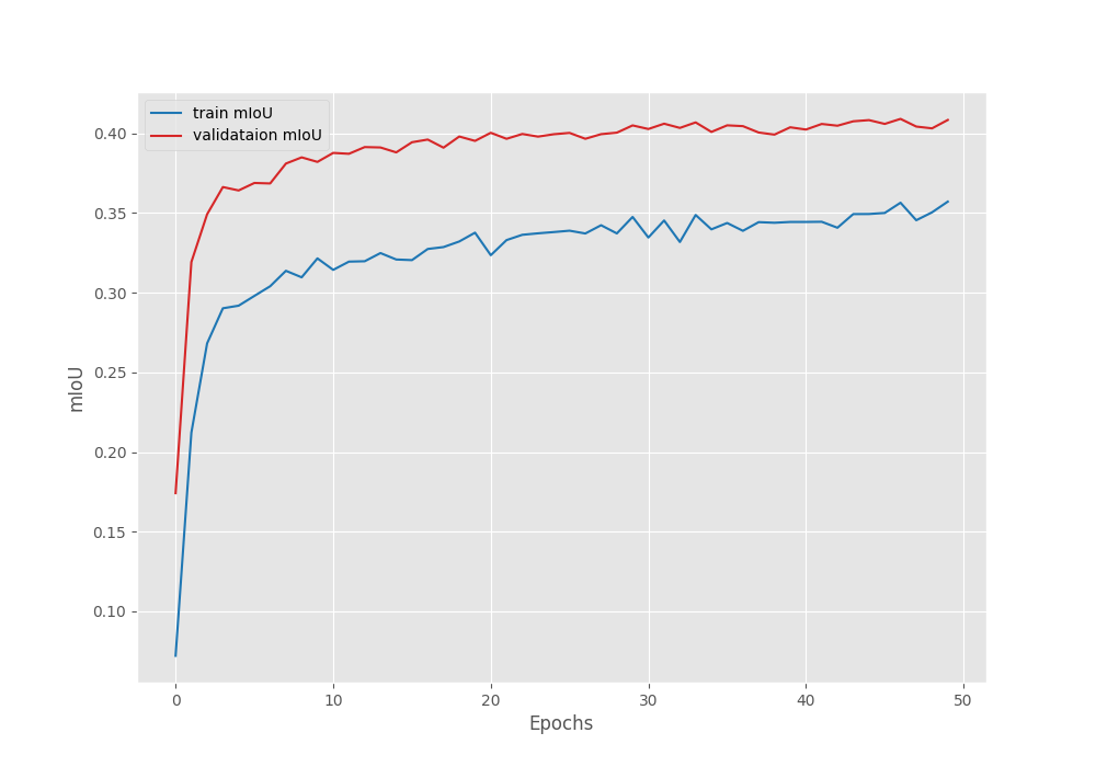
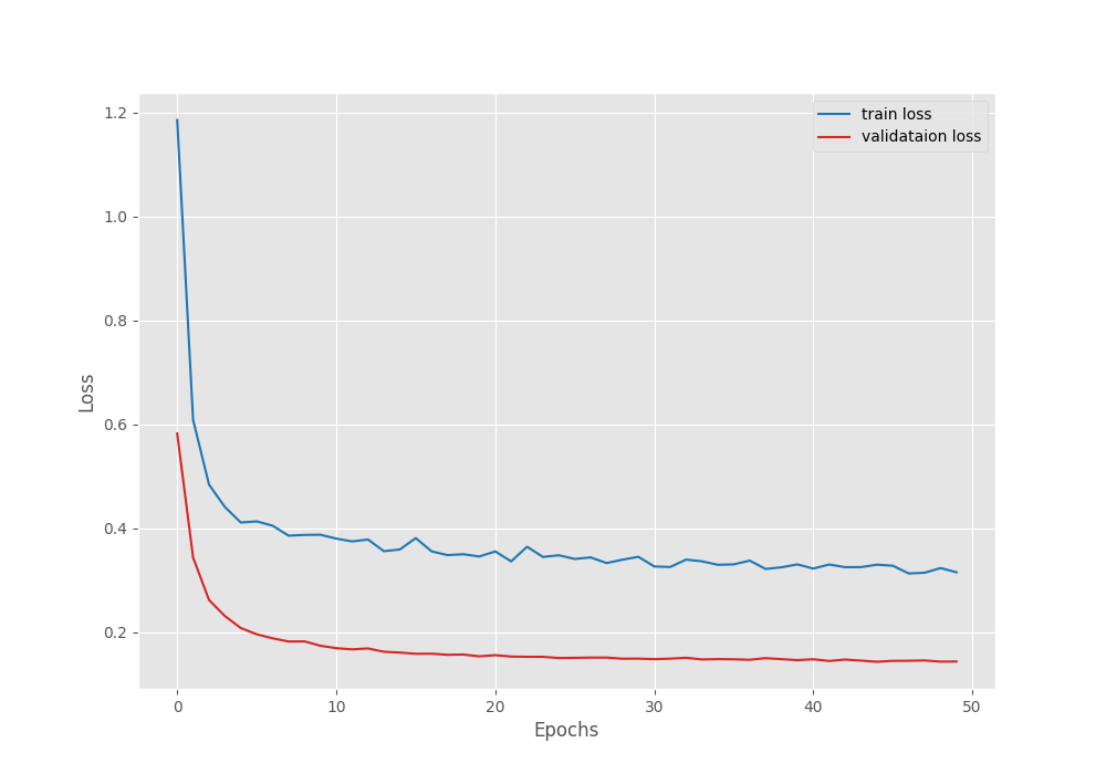
Transfer Learning DINOv3 Segmentation
We can execute the following command to start the transfer learning experiment.
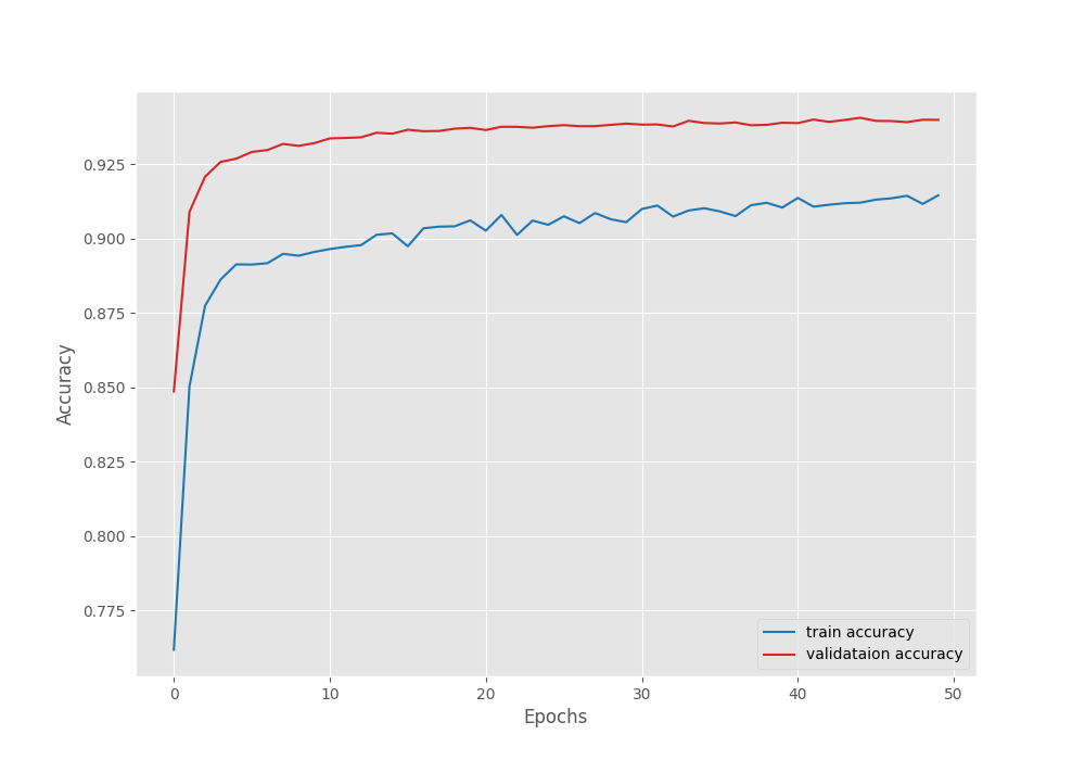
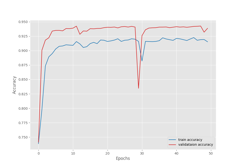
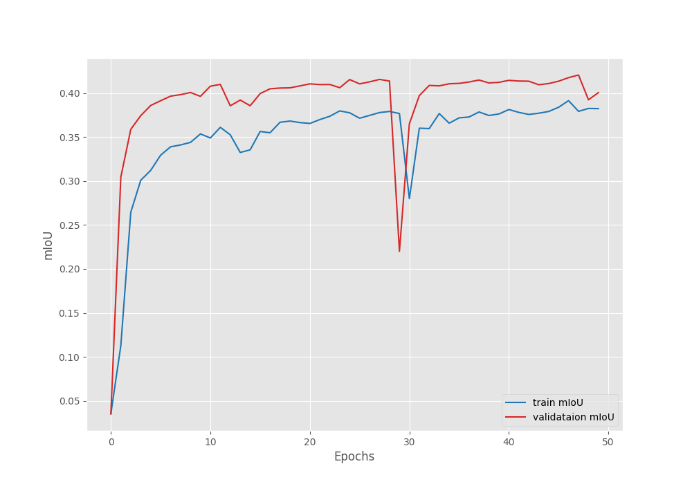
Compared to transfer learning, this time, the model reached a higher validation mean IoU of 42.04% on epoch 40. This shows that model can reach higher accuracy when training the backbone also.
Figure 7. Accuracy graph after fine-tuning the DINOv3 model on the Pascal VOC segmentation dataset.
Figure 8. Mean IoU graph after fine-tuning the DINOv3 model on the Pascal VOC segmentation dataset.
Figure 9. Loss graph after fine-tuning the DINOv3 model on the Pascal VOC segmentation dataset.
However, we can see an unusual dip in the validation plot in the above graphs. Furthermore, it is clear that the model has started to overfit quite early. Moreover, training the entire model requires more GPU memory as well. So, it is a tradeoff between slightly lower accuracy and speed of training each time we carry out these experiments. This will change from one use case to another.
Here, we will move forward with the better model from the fine-tuned experiment for running inference.
Inference Using the Trained DINOv3 Segmentation Model
We will start with the image inference code that is present in the infer_seg_image.py file. It is a simple codebase that loads the pretrained model, the configuration file, and goes through a directory of images to run inference.
We are using the following command line arguments here:
--input: This points to the directory containing the images.
--imgsz: The width and height of the images to resize to.
--model: Path to the pretrained weights.
--config: Path to the configuration file.
--model: Name of the model.
The results will be stored in outputs/inference_results_image directory. Here are the outputs.
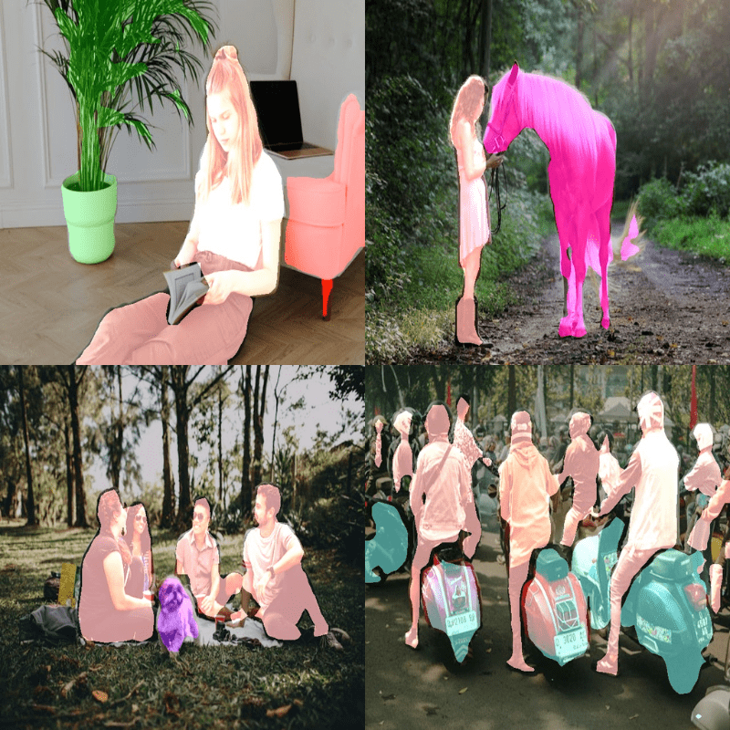
Figure 10. Image inference results after training DINOv3 segmentation model.
Overall, the model seems to be performing well. It is able to segment humans, vehicles, horses, and dogs. However, we can see sub-optimal masks when dealing with small and thin objects, such as the dog, the leaves of the plant, and the horse’s legs.
Let’s move on to the video inference. The code for this is present in image_seg_video.py.
The command line argument remains similar, with the only difference being that it points to a video rather than a directory of images.
The following is the result.
Video 1. Video inference result using the trained DINOv3 semantic segmentation model.
The results look good, but we can see some artifacts on the wheels of the bike and merging of the segmentation maps where the feet of the person are meeting the bike. On an RTX 3080 GPU, we are getting more than 76 FPS on average when running inference using the DINOv3 ViT-S/16 segmentation model.
Summary and Conclusion
In this article, we covered semantic segmentation training and inference using DINOv3. We started with the discussion of the dataset and codebase. Then we moved to converting the smallest DINOv3 Transformer backbone into a semantic segmentation model. This was followed by training, discussion of results, and inference.
If you have any questions, thoughts, or suggestions, please leave them in the comment section. I will surely address them.
You can contact me using the Contact section. You can also find me on LinkedIn, and X.
Liked it? Take a second to support Sovit Ranjan Rath on Patreon!
This website uses cookies so that we can provide you with the best user experience possible. Cookie information is stored in your browser and performs functions such as recognising you when you return to our website and helping our team to understand which sections of the website you find most interesting and useful.
Strictly Necessary Cookies
Strictly Necessary Cookie should be enabled at all times so that we can save your preferences for cookie settings.
If you disable this cookie, we will not be able to save your preferences. This means that every time you visit this website you will need to enable or disable cookies again.